For Beginners
v0.0.9, Copyright © February 11, 2023
This is an alpha-quality book. There are mistakes, oh yes. When you find them, please drop an issue in GitHub, or a pull request, or email me at beej@beej.us. When the number of defects gets low enough, I’ll offer a print version.
Hey, everyone! Have you been thinking about learning to program? Have you also been thinking of how to do it in the easy-to-approach Python programming language?
Yes? Then this is the book for you. We’re going to start with the absolute basics and build up from there, building up to being an intermediate developer and problem-solver! Python is the language we’ll be using to make this happen.
But by the end of the book, you will have developed programming techniques that transcend languages. After picking up Python, maybe try another language like JavaScript, Go, or Rust. They all have their own features to explore and learn.
Beginning programmers. If you have limited experience or no experience, this book is targeted at you!
Attitude Prerequisite: be inquisitive, curious, have an eye for puzzles and problem solving, and be willing to take on difficult challenges.
Technical Prerequisite: be a computer user. You know what files are, how to move them and delete them, what subdirectories (folders) are, can install software, and how to type.
Are you a seasoned developer looking to start with Python? I’m sorry but this is not likely to be the book you’re looking for. It will progress too slowly for your tastes. Just jump straight into the official Python documentation1.
I make an effort in this book to cover Mac, Windows, and Unix variants (via Arch Linux).
We’ll cover installing Python 3 and the Visual Studio Code editor. (Both are free.) If you already have a code editor you prefer using (Vim, Emacs, Sublime, Atom, PyCharm, etc.) feel free to use that. This book’s 100% certified editor agnostic!
The official location of this document is:
There you will also find example code.
I’m generally available to help out with email questions so feel free to write in, but I can’t guarantee a response. I lead a pretty busy life and there are times when I just can’t answer a question you have. When that’s the case, I usually just delete the message. It’s nothing personal; I just won’t ever have the time to give the detailed answer you require.
As a rule, the more complex the question, the less likely I am to respond. If you can narrow down your question before mailing it and be sure to include any pertinent information (like platform, compiler, error messages you’re getting, and anything else you think might help me troubleshoot), you’re much more likely to get a response. For more pointers, read ESR’s document, How To Ask Questions The Smart Way2.
If you don’t get a response, hack on it some more, try to find the answer, and if it’s still elusive, then write me again with the information you’ve found, and hopefully, it will be enough for me to help out.
Now that I’ve badgered you about how to write and not write me, I’d just like to let you know that I fully appreciate all the praise the guide has received over the years. It’s a real morale boost, and it gladdens me to hear that it is being used for good! :-) Thank you!
You are more than welcome to mirror this site, whether publicly or privately. If you publicly mirror the site and want me to link to it from the main page, drop me a line at beej@beej.us.
If you want to translate the guide into another language, write me at beej@beej.us and I’ll link to your translation from the main page. Feel free to add your name and contact info to the translation.
This source markdown document uses UTF-8 encoding.
Please note the license restrictions in the Copyright, Distribution, and Legal section, below.
If you want me to host the translation, just ask. I’ll also link to it if you want to host it; either way is fine.
Beej’s Guide to Python Programming is Copyright © 2019 Brian “Beej Jorgensen” Hall.
With specific exceptions for source code and translations, below, this work is licensed under the Creative Commons Attribution- Noncommercial- No Derivative Works 3.0 License. To view a copy of this license, visit
https://creativecommons.org/licenses/by-nc-nd/3.0/
or send a letter to Creative Commons, 171 Second Street, Suite 300, San Francisco, California, 94105, USA.
One specific exception to the “No Derivative Works” portion of the license is as follows: this guide may be freely translated into any language, provided the translation is accurate, and the guide is reprinted in its entirety. The same license restrictions apply to the translation as to the original guide. The translation may also include the name and contact information for the translator.
The C source code presented in this document is hereby granted to the public domain, and is completely free of any license restriction.
Educators are freely encouraged to recommend or supply copies of this guide to their students.
Unless otherwise mutually agreed by the parties in writing, the author offers the work as-is and makes no representations or warranties of any kind concerning the work, express, implied, statutory or otherwise, including, without limitation, warranties of title, merchantability, fitness for a particular purpose, noninfringement, or the absence of latent or other defects, accuracy, or the presence of absence of errors, whether or not discoverable.
Except to the extent required by applicable law, in no event will the author be liable to you on any legal theory for any special, incidental, consequential, punitive or exemplary damages arising out of the use of the work, even if the author has been advised of the possibility of such damages.
Contact beej@beej.us for more information.
Thanks to everyone who has helped in the past and future with me getting this guide written. And thank you to all the people who produce the Free software and packages that I use to make the Guide: GNU, Linux, Slackware, vim, Python, Inkscape, pandoc, many others. And finally a big thank-you to the literally thousands of you who have written in with suggestions for improvements and words of encouragement.
I dedicate this guide to some of my biggest heroes and inspirators in the world of computers: Donald Knuth, Bruce Schneier, W. Richard Stevens, and The Woz, my Readership, and the entire Free and Open Source Software Community.
This book is written in Markdown using the vim editor on an Arch Linux box loaded with GNU tools. The cover “art” and diagrams are produced with Inkscape. The Markdown is converted to HTML and LaTex/PDF by Python, Pandoc and XeLaTeX, using Liberation fonts. The toolchain is composed of 100% Free and Open Source Software.
Let’s say you’re entirely new to this stuff. You have a computer, you know how to use it, but you don’t know how to make it do exactly what you want it to.
It’s the difference between a user and a programmer, right?
But what does it mean to program a computer?
In a nutshell, you have a goal (what you want to compute), and programming is the way you get there.
A program is a description of a series of steps to complete that computation, blah blah blah…
Okay—instead think of a sequence of steps that you have to do to do anything. Like baking cookies for example.
Fun Computing Fact: everyone likes yummy cookies.
You often have that sequence of steps, that recipe, written down on a piece of paper. By itself, it’s definitely not cookies. But when you apply a number of kitchen implements and ingredients and an oven to it, pretty soon you have some cookies.
Of course, in that case, you have to do the work. With programming, the computer does the work for you. But you have to write down the recipe.
The recipe is the program. Programming is the act of writing down that recipe so the computer can execute it. And get those cookies baked.
Mmmm. Cookies.
Some programs are simple. “Add up these 12 numbers” is an example. It’s a breeze for the computer to do that.
But others are more complicated. They can extend into millions of lines long, or even tens of millions, written by large teams over many years. Think triple-A video game titles or the Linux operating system.
When you’re first starting, large programs like that seem impossible. But here’s the secret: each of those large programs is made up of smaller, well-designed building blocks. And each of those building blocks is made up of smaller of the same.
And when you start learning to be a programmer, you start with the smallest, most basic blocks, and you build up from there.
And you keep building! Writing software is a lifelong learning process. There are always new things to learn, new technologies, new languages, new techniques. It’s a craft to be developed and perfected over a lifetime. Sure, at first you won’t have that many tools in your toolkit. But every moment you spend working on software gives you more experience solving problems and gives you more methods to attack them.
In other words, I know what I want to see… how do I get there with the tools I know?
There’s a great scene in the movie Apollo 133 that I love. The CO2 scrubbers on the command module are spent, and the team wants to use the scrubbers from the lunar module to replace them. But the former are round, and the latter are square and won’t fit. Of course, the spacecraft has limited resources to repair it—just miscellaneous stuff on board that was meant for the mission.
On the ground, the team has all those items at hand, and they dump them on a table. A staff member holds up a square scrubber and a round scrubber and tells everyone, “We gotta find a way to make this fit into the hole for this.” He then gestures toward the table, adding, “Using nothing but that.”
And that’s what programming is like, except, obviously and fortunately no lives are at stake. (Typically.)
You have a limited set of programming techniques at your disposal, and you have the goal that you want to achieve. How can you get to that goal using only those tools? It’s a puzzle!
Fun Programming Fact: Most devs have no idea how to solve a problem when they’re first presented with it. They have to systematically attack it.
Programmers fully intend to use a well-reasoned approach to solving arbitrary problems. In reality, they often run off in high spirits and dive right into coding before they’ve done some of the very important preliminary work, but since they love programming so much they don’t seem to mind wasting time.
(And it’s not a waste of time because every second you’re programming, you’re learning!)
But lots of bosses do consider unplanned development to be a waste of time. Time is also known as “money” to the company that hired you. And the only thing more precious to a company than money is more money.
Imagine that you said, “I want to build an airplane!” and ran off an bought a pile of tools and metal and rivets and levers and started bolting it together immediately. You might find after a while that, oh you should have figured out how big the engine was before you built the fuselage, but, hey, no problem, you have time. You can just rebuild the fuselage. So you do. But now the canopy doesn’t fit. So you have to rebuild it again, and so on.
You could have saved a lot of time by actually planning what you were going to do before you started building.
It’s the same with software.
Fun Programming Proverb: Hours of debugging can save you minutes of planning.
There are several problem-solving frameworks out there. These are blueprints for how to approach a programming problem and solve it, even if you have no idea how to solve it when you first see it.
One of my favorite problem-solving frameworks was popularized by mathematician George Pólya in 1945 in his book How To Solve It. It was originally written for solving math problems, but it’s surprisingly effective at solving just about anything. The Four Main Steps are:
Understanding the Problem. Get clarity on all parts of the problem. Break it down into subproblems, and break those subproblems down. If you don’t understand the problem, any solutions you come up with will be solving the wrong problem! You know you understand the problem when you can explain it to someone completely.
Devising a Plan. How are you going to attack this with the tools you have at your disposal and the techniques you know? You know you’re done making a plan when you’re able to easily convert your plan into code.
Often when planning you realize there’s something about the problem you don’t fully understand. Just for a bit, pop back to Step 1 until it’s clear, then come back to planning.
Carrying out the plan Convert your plan into code and get it working.
Often in this phase, you find that there was either something you didn’t understand or something the plan didn’t account for. Drop back a step or two until it’s resolved, then come back here.
Looking Back. Look back on the code you got working, and consider what went right and what went wrong. What would you do differently next time? What techniques did you learn while writing the code? Was there any place you could have structured things better, or anyplace you could have removed redundant code?
What’s neat about this is that developers apply the steps of problem-solving to the entire program, and they also apply it to the smaller problems within the program. A big computing problem is always composed of many subproblems! The problem-solving framework is used within the problem-solving framework!
An example of a real-life problem might be “build a house”. But that’s made up of subproblems, like “build a foundation” and “frame the walls” and “add a roof”. And those are made up of subproblems, like “grade the lot” and “pour concrete”.
In programming, we break down problems into smaller and smaller subproblems until we know how to solve them with the techniques we know. And if we don’t know a technique to solve it, we go and learn one!
Being a developer is the same as being a problem solver. The problems ain’t easy, but that’s why it pays the big bucks.
So you should expect that any time you see a programming problem in this book, on a programming challenge website, at school, or work, that the answer will not be obvious. You’re going to have to work hard and spend a lot of time to get through the first problem-solving steps before you’ll even be ready to start coding.
Python is a programming language. This means it’s vaguely readable by humans, and completely readable by a machine. (As long as you don’t make the tiniest mistake!) This is a good combination, since people are bad at reading the actual 1011010100110 code that machines use. We use these higher-level languages to help us get by.
In this case, another piece of software called the Python interpreter takes the code we write in the Python language and runs it, performing the operations we’ve requested.
So before we begin, we need to install the Python interpreter. This is one of the most annoyingly painful parts of the whole book, but luckily it only has to be done once.
Okay, gang! Let’s get it… over with!
…I really need to work on the end of that inspirational speech.
Python is a programming language. It interprets instructions that you, the programmer, give it, and it executes them. Think of it like a robot you can give a series of commands to ahead of time, and then have it run off and do them on its own.
In programmer parlance, we call these sets of instructions code.
In addition to being a programming language, Python is also a program, itself! It’s a program that runs other programs! We don’t have to worry about the details of that at all, except that since Python is a program, it’s something we’ll have to install on our computers.
Python comes in different versions. The big versions are 2 and 3. We’ll be using Python 3 for everything in this book. Python 2 is older, and is rarely used in new projects.
Python also comes with an Integrated Development Environment, or IDE. An IDE is a program that helps you write, run, and debug (remove the errors from) code.
It’s main components are:
The editor. This is like a word processor except specifically designed for use with code.
The debugger. This helps you step through your code a line at a time and watch the data values change as you go. It can help you find places where your code is incorrect.
The console or terminal. This is a window where the output from your program appears (and where you might type input to the program).
The name of Python’s built-in IDE is IDLE. There are other IDEs we’ll talk about later.
There are two ways to do this:
I can’t see any disadvantage to installing it from the store. Just remember to install Python 3 (not Python 2).
If you install it from the official website4, you need to remember to check the “Add to PATH” box during the install procedure!
Another option to installing Python on Windows is through WSL. We’ll cover this later.
Download and install Python for Mac from the official website5.
Another option to installing Python on Mac is through Homebrew. We’ll cover this later.
The Linux community tends to be pretty supportive of people looking to install things. Google for something like ubuntu install python3, replacing ubuntu with the name of your distribution.
Here’s where we get to run the IDE for the first time. First we’ll look at how to do it on various platforms, and then we’ll run some Python code in it.
Running IDLE depends on the platform:
| Platform | Commands |
|---|---|
| Windows | Hit the Start menu and type “idle”. It should show up in the pick list and you can click to open it. |
| Mac | Hit CMD-SPACE and type “idle”. It should show up in the pick list and you can click to open it. |
| Unix-like | Type idle in the terminal or find it in your desktop pulldown menu. |
If you run idle on the command line and it says something about the command not being found, try running idle3.
If you get an error on the command line that looks like this:
** IDLE can't import Tkinter.
Your Python may not be configured for Tk. **
you’ll have to install the Tk graphical toolkit. This might be a package called tk or maybe python-tk. If you’re on a Unix-like, search for how to install on your system. On a Mac with Homebrew, you can brew install python-tk.
If you get another error, cut and paste that error into your favorite search engine to see what other people say about how to solve it.
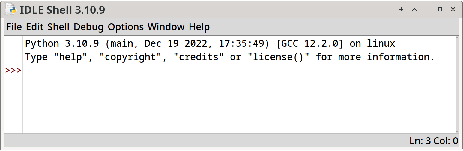
Once IDLE is up, you should see a window that looks vaguely like this:
In the IDLE window after the >>> prompt, type:
print("Hello, world!")and hit RETURN. This commands Python to output the words “Hello, world!”.
>>> print("Hello, world!")
    Hello, world!
And it did!
This is just the beginning!
Let’s use our problem-solving framework!
Understand the Problem: We want to write a program that prints a neat little message to the screen.
Devise a plan
Carry out the Plan: This is where we execute our plan. We’ll do that in the following sections.
Look Back: We’ll do this, below, as well. In future chapters, we’ll leave these last two off the number list and just do them in subsequent sections.
Let’s go!
Run IDLE as discussed in the previous chapter.
Once in there, we’re going to make a new file.
It used to be that everyone who used computers knew what a file was. But these days, many people use computers for years without encountering the concept.
So! A file is a collection of data with a name. Examples of files would be images, movies, PDF documents, music files, and so on.
The name indicates something about the contents of the file. Generally. It really can be anything, but that would be misleading, like labeling a box of raisins as “Chocolate”.
The name is split into two parts, commonly, separated by a period. The first part is the name, and the second part is the extension. Confusingly sometimes people refer to the name and extension together as the “name”, so you’ll have to rely on context.
Sometimes, depending on the system, the extension is optional.
As an example, here’s a complete file name and extension:
{.default} hello.pyThere we have a file named
helloand an extension.py. This is a common extension that means “this is a Python source code file”.
Pull down “File→New” and that’ll bring up a blank window.
And let’s enter some code!
Type the following6 into the editor (the line numbers, below, are for reference only and shouldn’t be typed in):
We’re (almost) ready to run!
Hit F5 from the editor window (you might have to hit fn-F5 on the Mac) to run the code. Alternately, you can pull down the “Run” menu and select “Run Module”.
If you haven’t saved the file, it will prompt you to save the file. (You can pull down “File→Save”, or hit COMMAND-S or CTRL-S to do this preemptively.)
Give it a good name, like hello.py.
And then, in the console window, you’ll see the output appear! [Angelic Chorus!]
Hello, world!
My name's Beej and this is (possibly) my first program!
Did you miss it? Hit F5 again and you’ll see it appear again.
You just wrote some instructions and the computer carried it out!
Next up: write a Quake III clone!
Okay, so maybe there might be a small number of in between things that I skimmed over, but, as Obi-Wan Kenobi once said, “You’ve taken your first step into a larger world.”
Remember to use the four problem-solving steps to solve these problems: understand the problem, devise a plan, carry it out, look back to see what you could have done better.
dijkstra.py that prints out your three favorite Edsger Dijkstra quotes7.For this chapter, we want to write a program that reads two numbers from the keyboard and prints out the sum of the two numbers.
Problem-solving step: Understanding the Problem.
Data is the general term we use to describe information stored in the computer. In the case of programming, we’re interested in values that we’ll do things with. Like add together. Or turn into a video game.
Really, data is information. Can you glean information from a symbol? Then it’s data. Sometimes it’s a symbol like “8”, or maybe a string of symbols like “cat”.
Your goal as a software developer is to write programs that manipulate data. You have to manipulate the input data in such a way that the desired output is achieved. And you have to solve the problem of how to do that.
In a program, data is commonly stored in what we call variables. If you’ve taken any algebra, you are familiar with a letter that holds the place of a value, such as the “slope-intercept” form of the equation of a line:
\(y = mx + b\)
or of a parabola:
\(y = x^2\)
But beware! In programming code, variables don’t behave like mathematical equations. Similar, but different.
Enter the following code in a new program in your editor, save it, and give it a run. (This is just like you did with the program in the earlier chapter. You can name this one anything you’d like. If you need inspiration, vartest.py8 seems good to me.)
In Python, variables refer to values9. We’re saying on line 1 of the code, above, “The variable x refers to the value 34.” Another way to think of this that might be more congruent with other languages is that x is a bucket that you can put a value in.
Then Python moves to the next line of code and runs it, printing 34 to the screen. And then on line 3, we put something different in that bucket. We store 90 in x. The 34 is gone–this type of bucket only holds one thing10.
So the output will be:
34
90You can see how the variable x can be used and reused to store different values.
We’re using
xandyfor variable names, but they can be made up of any letter or group of letters, or digits, and can also include underscores (_). The only rule is they can’t start with a digit!These are all valid variable names (and, of course, you can make up any name you want!):
y a1b2 foo Bar FOOBAZ12 Goats_Rock
You can also do basic math on numeric variables. Add to the code above:
x = 34      # Variable x is assigned value 34
print(x)
x = 90      # Variable x is assigned value 90
print(x)
y = x + 40 # y is assigned x + 40 which is 90 + 40, or 130
print(x) # Still 90! Nothing changed here
print(y) # Prints "130"On line 6, we introduced a new variable, y, and gave it the value of “whatever x’s value is plus 40”.
What are all these
#marks in the file? We call those hash marks, and in the case of Python, they mean the rest of the line is a comment and will be ignored by the Python interpreter.
One last important point about variables: when you do an assignment like we did, above, on line 6:
y = x + 40 # y is assigned 130When you do this, y refers to the value 130 even if x changes later. The assignment happens once, when that line is executed, with the value in x at that snapshot in time, and that’s it.
Let’s expand the example farther to demonstrate:
x = 34      # Variable x is assigned value 34
print(x)
x = 90      # Variable x is assigned value 90
print(x)

y = x + 40  # y is assigned x + 40 which is 90 + 40, or 130
print(x)    # Still 90! Nothing changed here
print(y)    # Prints "130"
x = 1000
print(y) # Still 130!Even though we had y = x + 40 higher up in the code, x was 90 at the time that code executed, and y is set to 130 until we assign into it again. Changing x to 1000 did not magically change y to 1040.
Fun Tax Fact: The 104011 is nearly my least-favorite tax form.
For more math fun, you have the following operators at your disposal (there are more, but this is enough to start):
| Function | Operator |
|---|---|
| Add | + |
| Subtract | - |
| Multiply | * |
| Divide | / |
| Integer Divide12 | // |
| Exponent | ** |
You can also use parentheses similar to how you do in algebra to force part of an expression to evaluate first. Normal mathematical order of operations rules apply13.
 8 + 4  / 2   #  8 + 4  / 2 ==  8 + 2 == 10
(8 + 4) / 2   # (8 + 4) / 2 == 12 / 2 == 6
And you thought all that algebra wouldn’t be useful… pshaw!
There’s a common pattern in programming where you want to, say, add 5 to a variable. Whatever value it has now, we want to make it 5 more than that.
We can do this like so:
x = 10

x = x + 5   # x = 10 + 5 = 15
This pattern is so common, there’s a piece of shorthand14 that we can use instead.
These two lines are identical:
x = x + 10
x += 10
As are these:
x = x / 5
x /= 10
Here are a few of the arithmetic assignment expressions available in Python:
| Operator | Meaning | Usage |
|---|---|---|
+= |
Add and assign | x += y |
-= |
Subtract and assign | x -= y |
*= |
Multiply and assign | x *= y |
/= |
Divide and assign | x /= y |
%= |
Modulo and assign | x %= y |
These are very frequently used by devs. If you have x = x + 2, use x += 2, instead!
Let’s check out this code:
x = 1000
y = x
Something interesting happens here that I want you to make note of. It’s not going to be super useful right now, but it will be later when we get to more intermediate types of data.
When you do this, both x and y refer to the same 1000.
That’s a weird sentence.
But think of it this way. Somewhere in the computer memory is the value 1000. And both x and y refer to that single value.
If you do this:
x = 1000
y = 1000
Now there are two 1000 values. x points to one, and y points to the other.
Finally, adding on to the original example:
x = 1000
y = x
y = 1000
What happens there is that first there is one 1000, and x refers to it.
Then we assign x into y, and now both x and y refer to the same 1000.
But then we assign a different 1000 to y, so now there are two 1000s, referred to by x and y, respectively.
(The details of this are rather more nuanced than I’ve mentioned here. See Appendix C if you’re crazy enough.)
Takeaway: variables are just names for items in memory. You can assign from one variable to another and have them both point to the same item.
We’re just putting that in your brain early so that we can revive it later.
Problem-solving step: Understanding the Problem.
This is a biggie, so listen up for it.
When you’re programming, it’s important to keep a mental model of what should happen when this program runs.
Let’s take our example from before. Step through it in your head, one line at a time. Keep track of the state of the system as you go:
Before we begin, x has no value. So represent that in your head as “x has no value; it’s invalid”.
Then the first line runs.
x is now 34.
Then the second line runs.
x is still 34, and we print it out. (So 34 is printed.)
Then the third line runs.
x is no longer 34. It is now 90. 34 is gone.
Then the fourth line runs.
x is still 90, and 90 gets printed out.
Then we’re out of code, so the program exits. And we have “34” and “90” on the screen from when they were printed.
That’s keeping a mental model of computation.
This is the key to being able to debug. When your mental computing model shows different results than the actual program run, you have a bug somewhere. You have to dig through your code to find the first place your mental model and the actual program run diverge. That’s where your bug is.
Problem-solving step: Understanding the Problem.
We want to get input from the user and store it in a variable so that we can do things with it.
Remember that our goal in this chapter is to write a program that inputs two values from the user on the keyboard and prints the sum of those values.
Python comes with a built-in function that allows us to get user input. It’s called, not coincidentally, input().
But wait—what is a function?
A function is a chunk of code that does something for you when you call it (that is when you ask it to). Functions accept arguments that you can pass in to cause the function to modify its behavior. Additionally, functions return a value that you can get back from the function after it’s done its work.
So here we have the input() function15, which reads from the keyboard when you call it. As an argument, you can pass in a prompt to show the user when they are ready to type something in. And it returns whatever the user typed in.
What do we do with that return value? We can store it in a variable! Let’s try!
Here’s another program, inputtest.py16:
# Take whatever `input()` returns and store it in `value`:

value = input("Enter a value: ")
print("You entered", value)
We can run it like this:
$ python3 inputtest.py
Enter a value: 3490
You entered 3490
Check it out! We entered the value 3490, stored it in the variable value, and then printed it back out! We’re getting there!
But you can also call it like this:
$ python3 inputtest.py
Enter a value: Goats rock!
You entered Goats rock!
Hmmm. That’s not a number. But it worked anyway! So are we all good to go?
Yes… and no. We’re about to discover something very important about data.
Problem-solving step: Understanding the Problem.
We started with numbers, earlier. That was pretty straightforward. The variable was assigned a value and then we could do math on it.
But then we saw in the previous section that input() was returning whatever we typed in, including Goats rock! which is certainly not any number I’ve ever heard of.
And, no, it’s not a number, indeed. It’s a sequence of characters, which we call a string. A string is something like a word, or a sentence, for example.
Wait… there’s another type of data besides numbers? Yes! Lots of types of data! We call them data types.
Python associates a type with every variable. This means it keeps track of whether a variable holds an integer, a floating point17 number or a string of characters.
Here are some examples and their associated types. When you store one of these values in a variable, the variable remembers the type of data stored within it.
| Example Data | Type in English | Type name in Python |
|---|---|---|
2 |
Integer | int |
3490 |
Integer | int |
-45 |
Integer | int |
0 |
Integer | int |
3.14159 |
Floating Point | float |
-13.8 |
Floating Point | float |
0.0 |
Floating Point | float |
"Hello!" |
String | str |
"3490" |
String | str |
"" |
String (empty) | str |
In the examples, above, strings are declared using double quotes ("), but they can also be done with single quotes, as long as the quotes match on both ends:
"Hello!"  # is the same as 'Hello!'
'Hello!'  # is the same as "Hello!"
Okay, that’s all fine. But is input() returning a string or a number? We saw both happen when we tried it out, right?
Actually, turns out, input() always returns a string. Period. Even if that’s a string of numbers. Note that these things are not the same:
3490     # int, a numeric value we can do math with
"3490"   # string, a sequence of characters
Sure, they look kinda the same, but they aren’t the same because they have different types. You can do arithmetic on an int, but not on a string.
Well, that’s just great. The task for this chapter is to get two numbers from the keyboard and add them together, but the input() function only returns strings, and we can’t add strings together numerically!
How can we solve this problem?
Problem-solving step: Understanding the Problem.
If we can’t add strings mathematically, can we convert the string "3490" into the integer 3490 and then do math on that?
Yes!
In fact, we can convert back and forth between all kinds of data types! Watch us convert a string to a number and store it in a variable:
a = "3490"    # a is a string "3490"
b = int(a)    # b is an integer 3490!

print(b + 5)  # 3495
How did that work? We called the built-in int() function and passed it a string "3490". int() did all the hard work and converted that string to an integer and returned it. We then stored the returned value in y. And finally, we printed the value of b+5 just to show that we could do math on it.
Perfect!
Here are some of the conversion functions available to you in Python:
| Function | Effect |
|---|---|
int() |
Convert argument to an integer and return it |
float() |
Convert argument to a floating-point number and return it |
str() |
Convert argument to a string and return it |
So… given all that we know so far, how can we solve this chapter’s problem: input two numbers from the keyboard and print the sum?
Problem-solving step: Devising a Plan.
We know:
Now—how do we put all that together to write a program that inputs two numbers from the keyboard and prints their sum?
This is the Devising a Plan portion of problem-solving. We’re not going to write code to make this happen. We’re just going to write an outline of the individual steps the program must describe in a language called pseudocode (which is English that looks kinda like code).
Then when we’re satisfied it’ll work, we can code it up for realsies.
So stop here and take a moment to consider what the step by step might be to get this done.
Really, take a moment, because I’m about to give spoilers. Thinking about how to solve problems is 80% of what a software developer gets paid to do, so you might as well practice right now.
What do we know? What tools do we have at our disposal? What resources? How do I put all those together to solve this problem, like solving a puzzle?
Here’s some pseudocode that would get the job done, it looks like:
read string from keyboard into variable x
convert x to int and store it back in x again
read string from keyboard into variable y
convert y to int and store it back in y again
print the sum of x + y
If we’re satisfied that our plan is solid, it’s time to move to the next phase.
Problem-solving step: Carrying out the Plan.
Now let’s convert each of those lines to real Python. I’ll throw in the pseudocode as comments so we can see how they compare. (Source code link18.)
# Read string from keyboard into variable x
x = input("Enter a number: ")

# Convert x to int and store it back in x again
x = int(x)

# Read string from keyboard into variable y
y = input("Enter another number: ")

# Convert y to int and store it back in y again
y = int(y)

# Print the sum of x + y
print("The sum of the two numbers is:", x + y)
Save that file as twosum.py and run it:
$ python3 twosum.py
Enter a number: 9
Enter another number: 8
The sum of the two numbers is: 17
Too easy! Let’s challenge it:
$ python3 twosum.py
Enter a number: 235896423496865928659832536289
Enter another number: 94673984675289643982463929238
The sum of the two numbers is: 330570408172155572642296465527
Not even breaking a sweat!
Nice. Now, I want you to think like a villain. What would a villain pass into our program for input that would cause it to break?
Try all those things with your program. What happens when you try it? Which ones work and which ones don’t?
Notice that a big, spewing error message is really the worst case scenario here. And it’s not really that painful. Don’t be afraid to try to break your code. The computer can handle it. Just run it again.
Later, we’ll learn techniques to catch errors like this so that the program doesn’t bomb out, and prints a nice message to the user to please try again with valid input, thank you very much.
Notice that when the program crashes, buried in all that output, is the line number the program crashed on! Very, very useful! And the last line tells you exactly what Python thinks went wrong.
The point is, if you’re not sure how something will work, just try it. Experiment! Break things! Fix things! Again, the computer can absolutely handle it. It’s just a big sandbox for you to play in.
Problem-solving step: Looking Back.
This grimly-named step is where we take a look at our code and decide if there was a better way to attack this problem. It’s important to remember that coding is a creative endeavor. There are many ways to solve the same problem.
Admittedly, right now, you don’t have many tools in the toolkit, so your creativity is limited. But eventually, in the not-too-distant future, you’ll know several ways to solve a problem, and you’ll have to weigh the pros and cons of each, and be creative and choose one!
What could be better?
What else could we do?
“You know how to get to Carnegie Hall?”
“Practice!”
Zeus says, “This book assumes you complete all of the exercises!” and when Zeus speaks, people really should listen.
I know, I know. You get to the exercises part of a book and you just skip ahead. I mean, it’s not like I’m grading you or anything.
But there’s only one way to get to be a better dev: practice and repetition. Going through this book without doing the exercises is like training for a marathon by reading about how to run. It’s simply not going to get you there on its own.
Resist the urge to look at the solution until you’ve solved it! Give yourself a time limit. “If I haven’t solved this in 20 minutes, I can look at the solution.” That 20 minute isn’t wasted—it’s invaluable problem-solving practice time. During that time, you’re building a scaffold in your brain that can hold the solution once you see it.
If you just skip straight to the solution, look at it, and say, “Yup, makes sense, I got it,” you’re missing out on all that benefit.
Don’t shortchange yourself! Do the exercises! The more you do, the better dev you’ll be! I’m getting off my soapbox now!
Remember to use the four problem-solving steps to solve these problems: understand the problem, devise a plan, carry it out, look back to see what you could have done better.
Here they are:
Make a version of the two number sum code that works with floats instead of ints. Do the numbers always add correctly, or are they sometimes just a little bit off? Lesson: floating point math isn’t always exact. Sometimes it’s off by a tiny fraction. (Solution19.)
Have the program print out the sum and the difference between two numbers. (Solution20.)
Allow the user to enter 3 numbers and perform the math on those. (Solution21.)
Write a program that allows the user to enter a value for \(x\), and then computes and prints \(x^2\). Remember ** is the exponentiation operator in Python. 3**2 is 9. (Solution22.)
Write a program that allows the user to enter a, b, and c, and the solves the quadratic formula23 for those values.
A refresher: with equations of the form:
\(ax^2+bx+c=0\)
you can solve for \(x\) with the quadratic formula:
\(x=\cfrac{-b\pm\sqrt{b^2-4ac}}{2a}\)
This all looks terrifying! Can you feel your brain seizing up over it? Deer in the headlights? That’s OK. This is how developers feel when confronted with a new problem. Really! All of us! But what we know is that we have a problem solving framework we can use to attack this problem regardless of how difficult it seems initially.
Remember: Understand, Plan, then Code It Up.
Take a deep breath. Shake off the fear!
You can absolutely do this. It’s not any harder than anything so far! Let’s go!
Your program should plug a, b, and c into the above formula and print out the result value in x.
Make sure \(b^2\ge4ac\) or there won’t be a solution and you’ll get a “domain error” when you try to take the square root of a negative number. Some test values for \(a\), \(b\), and \(c\) that work:
5,9,3, or20,140,60.
What is that \(\pm\) symbol after \(-b\) in the equation? That’s “plus or minus”. It means there are actually two equations, one with \(+\) and one with \(-\):
\(x_{plus}=\cfrac{-b+\sqrt{b^2-4ac}}{2a}\) \(x_{minus}=\cfrac{-b-\sqrt{b^2-4ac}}{2a}\)
Solve them both and print out both answers for a given \(a\), \(b\), and \(c\).
What about that square root of \(b^2-4ac\)? How do you compute that? Here’s a demo program for computing the square root of 2—use it to learn how to use the math.sqrt() function, and then apply it to this problem.
import math      # You need this for access to the sqrt() function

x = math.sqrt(2) # Compute sqrt(2)
print(x)         # 1.4142135623730951
Code that up and, hey! You’ve written a program that solves quadratic equations! Take that, homework! (Solution24.)
Followup to the previous question: after computing x, go ahead and compute the value of
\(ax^2+bx+c\)
and print it out. (You can use either the plus solution or the minus solution—doesn’t matter since they’re both solutions.) The result should be exactly 0. Is it? Or is it just something really close to zero? Lesson: floating point math isn’t always exact. Sometimes it’s off by a tiny fraction.
Sometimes you might get a number back that looks like this, with a funky e-16 at the end (or e-something):
8.881784197001252e-16
That’s a floating point number, but in scientific notation25. That e-16 is the same as \(\times10^{-16}\). So the math equivalent is:
\(8.881784197001252\times10^{-16}\)
Now, \(10^{-16}\) is actually a really, really small number. So if you see something like e-15 or e-18 at the end of a float, think “that’s a really small number, like close to zero.”
Make up two more exercises and code them up.
And don’t worry–we’ll get away from the math examples soon enough. It’s just, for now, that’s about all we know. More soon!
This chapter we covered:
It’s a great start, but there’s plenty more to come!
if statementswhile loopfor loop and range iteratorFor this chapter, we want to write a program that asks the user for a number between 5 and 50, inclusive.
If a number outside that range is entered, an error message is printed and the user is asked again to enter a valid number.
Once the number is obtained, the program will print out that many # characters in a row. EXCEPT all characters at position 31 and above should print out a *. (Characters before that position will still be a #.)
For example, an input of 10 would result in:
##########whereas an input of 37 would result in:
##############################*******Keep this program in mind as we learn the techniques to implement it.
Problem-solving step: Understanding the Problem.
What is flow control? To understand, let’s look at a simple program:
When this program runs, Python keeps track of the current instruction, or line, if you will.
First, Python runs the first line.
Then it goes to the next.
Then it goes to the last.
And then it falls off the end and completes.
Kind of monotonous, right? I mean, it just brainlessly goes to the next instruction every time.
What if you want to transfer the program flow elsewhere instead of just blindly going to the next instruction?
This is where you get your first taste of what it means to be a developer. You can ask the computer to make smart decisions based on the criteria you specify. Figuring out which criteria to specify is the job of a programmer and where most of the hard work comes in.
Eventually, we’re going to code up things that say “If some condition is true, do one thing” or “If some condition is false, do another thing”.
But before that, we have to meet someone: George Boole.
Problem-solving step: Understanding the Problem.
George Boole27 was quite an interesting character. From humble beginnings in the early 1800s, he went on to develop the mathematics that became, in many ways, the foundation of modern computation. Pretty awesome.
What he developed is what we call today Boolean Algebra.
Don’t worry–it’s easier than that algebra you’re thinking of. In fact, you already know it, just not formally and not by that name.
With Boolean, we’re interested in whether or not expressions are true or false. And then we can make decisions on whether or not they are.
Let’s do some human ones before we get into the computer stuff.
Level: Easy. Are these expressions true or false for you?
Hopefully, that wasn’t particularly challenging. Let’s take it up a notch by introducing the concept of AND. For these, the entire expression is true only if all subexpressions are true.
For example, the statement “I’m over 190 cm tall AND I’m under 30 years of age” is false. Though I am over 190 cm tall, am I not under 30 years, so the entire expression is false.
By comparison, “I like dogs AND I like motorcycles” is true, because both of those subexpressions are true.
And if neither of them is true, the result is also false.
Level: Intermediate. Are these expressions true or false for you?
All right! Let’s do a variant on AND, namely OR. With OR, the entire expression is true if either or both of the subexpressions is true.
For example, I don’t like running, but I do like bicycling. Nevertheless, the following statement is true, because at least one of the subexpressions is true: “I like running OR I like bicycling”. True.
This is the basis for the smarty-pants answer to the question:
“Would you like soup or salad?”
“True. I would like soup or I would like salad.”
“Get out of my restaurant, Boolean fanatic!”
Level: Intermediate. Are these expressions true or false for you?
All right! Now one more thing to remember: unless there are parentheses in an expression saying otherwise, AND takes precedence over OR. That is, do the ANDs first, and then do the ORs.
Level: Advanced.
Let’s say it’s raining, I’m over 25, and this fish is big. We could evaluate this expression:
It’s sunny AND this fish is big OR I’m over 25.
We do the AND first. It’s not sunny, and the fish is big. So that’s “false AND true”, which evaluates to “false”.
So replace that AND expression with “false”. And then we’ll do the OR:
false OR I’m over 25.
Now I am over 25, so that evaluates to “false OR true”, which is “true”.
So the entire expression is true.
And you can override with parentheses:
It’s sunny AND (this fish is big OR I’m over 25).
Do the work in parens first. So now we evaluate the OR, which evaluates to “true OR true” which is “true”. Then we evaluate the AND, which is “It’s sunny AND true”, which is “false AND true”, which is “false”.
So the entire expression is false.
Let’s do some examples with numeric conditional expressions. Do these evaluate to true or false?
Answers:
Sometimes developers (but more usually hardware folks) describe these operations in what are called truth tables. A truth table shows what the result of a Boolean expression will be for some given inputs.
Often these tables use 1 to represent True and 0 to represent False28.
Here are some truth tables for the operations we’ve seen so far.
| A | B | A AND B |
|---|---|---|
0 |
0 |
0 |
0 |
1 |
0 |
1 |
0 |
0 |
1 |
1 |
1 |
| A | B | A OR B |
|---|---|---|
0 |
0 |
0 |
0 |
1 |
1 |
1 |
0 |
1 |
1 |
1 |
1 |
| A | NOT A |
|---|---|
0 |
1 |
1 |
0 |
Now we’re about ready to go. Let’s learn how to do this in Python.
Problem-solving step: Understanding the Problem.
The comparison operators in Python are:
| Operator | Effect |
|---|---|
< |
Less than, e.g. x < y |
> |
Greater than, e.g. x > y |
== |
Equal to, e.g. x == y |
!= |
Not equal to, e.g. x != y |
<= |
Less than or equal to, e.g. x <= y |
>= |
Greater than or equal to, e.g. x >= y |
So we can take a variable and convert it to a true or false value by comparing it to numbers or other variables.
What is true and false in Python?
| Boolean | Python Keyword |
|---|---|
| True | True |
| False | False |
Easy enough.
print(True)     # True
print(False)    # False

x = 10
print(x == 10)  # True
print(x < 5)    # False

# You can store the Boolean result in a variable!
r = x >= 7
print(r)        # True
Check that out! You can store the Boolean result of a comparison in a variable, like we did with r, above!
It’s important to note that True and False are not strings. They represent Boolean values.
So now, for data types, we know about strings, ints, floats, and Booleans (sometimes called bools for short). Add that to the collection of tools we have at our disposal.
But what about our good friends AND and OR?
| Boolean | Python Keyword |
|---|---|
| AND | and |
| OR | or |
| NOT | not |
Pretty easy, but I threw in a NOT! What is that? It’s pretty easy: it just inverts whatever you give it. “NOT true” is false. And “NOT false” is true.
print(not False) # Prints TrueSeems mundane, but we’ll make good use of it in a minute.
if StatementProblem-solving step: Understanding the Problem.
It’s all well and good for Python to tell me that 1 < 5 is True, but how can we actually use that to make choices in a program?
Let’s consider a small program that will let the user input a number and it will tell the user if the number is between 50 and 59, inclusive.
Before coding, let’s think about how to approach it. If the number is stored in x, what would the Boolean expression in Python be that would be True if x were between 50 and 59?
I’m talking ands and ors and nots and <s and >s… not necessarily all of them, but the ones needed.
Did you get it? Spoilers ahead!
x >= 50 and x <= 59 # True if x in that range!Let’s take that knowledge and turn it into a complete program30 using if, and then we can take it apart in more detail:
x = input("Enter a number: ")
x = float(x)

if x >= 50 and x <= 59:
    print(x, "is between 50 and 59, inclusive")
    print("Well done!")
else:
    print(x, "is not between 50 and 59, inclusive")
So if x >=50 and x <= 59 is True, then we execute the block that is indented afterward.
Blocks can be indented with any combination of tabs or spaces, as long as each line in the block begins with the same pattern of tabs or spaces. The official recommendation is to use 4 spaces for indentation in Python.
Indented blocks in Python are one of the things most devs are pretty opinionated about in terms of loving or hating. Personally, I say be a good dev in any language, regardless of how you feel about their idiosyncrasies.
And then what’s this pesky else? That’s a super-handy feature of if. If the condition is False, then the block under the else is evaluated instead. Basically, we’re saying, “If the condition is true, then do this, otherwise do this.”
There’s one more construct we can use in the if-else family: elif. This is short for else if and is used if you need to check multiple conditions.
if x < 10:
    print("x is less than 10")
elif x < 20:
    print("x is less than 20")
elif x < 30:
    print("x is less than 30")
else:
    print("x is greater than or equal to 30")
In that example, first we check if x is less than 10. If that’s False, the next condition is tested, and so on. If none of them match, then we get to the else case.
The if statement is the core of what allows us to use Boolean logic to control the flow of our program. It’s how computers can make decisions based on input. Without if, there would be no computing–that’s how important it is!
And your job as a dev is to come up with that logic, those if statements and conditions, that cause your program to give the proper output for a given input.
while Loops!Problem-solving step: Understanding the Problem.
We’re going to divert ever-so-slightly, and talk about another important concept in programming: loops. A loop is what allows us to execute the same piece of code repeatedly without repeating ourselves.
Here’s a real-life example. Let’s say you have to add some shingles to a roof. The steps to do so are to place a shingle, nail it in place, and then move to the next spot.
Instructions for four shingles might be:
But that’s irksomely verbose. It would be nicer to do something like this:
That’s us looping. We’re running the same piece of code while a condition is True. At the very least, this can save us a lot of typing!
Python has several looping statements, but for this section, we’ll concentrate on what’s called the while-loop. It does something while a condition is true.
Here’s an example31 that counts from 1200 to 1210:
It repeats the body of the loop (everything that’s indented) as long as the condition x <= 1210 is True.
You see inside the body of the loop, we increment (add one to) x every iteration so that it increases toward 1210.
What would happen if we didn’t increment x? In that case, it would loop forever. We call this an infinite loop. If your program’s running for a long time with no output (or repeating output), it might be in an infinite loop.
How do you get out of your program if it’s caught in an infinite loop? You hit CTRL-C (AKA “break”). That’ll get you back to your shell prompt.
Remember one of our goals for this chapter’s program is to ask the user for a number between 5 and 50. And we need to ask them again if they enter a number outside that range. That is, we need to loop while the user has not given us valid input. Give that some thought now, and we’ll come back to it later.
for LoopsProblem-solving step: Understanding the Problem.
In addition to while loops, we also have a beast called a for loop. These are quite powerful as we’ll find out later, but for now, I just want to talk about looping for a certain number of times. (As opposed to looping while a condition is true.)
Here’s an example of printing out the numbers from 0 to 9 using a for loop and a function called range(). (range() returns something called an iterator. More on iterators in upcoming chapters—for now, just look at how they can be used with for loops.)
for i in range(10):  # loop from 0 to 9
    print(i)
Notice a few things:
i is the classic variable name for a looping index.j, then k, etc.range(). Up to but not including.But wait, there’s more! range() is multi-talented! Not only can it count up from zero to almost-a-number, but you could give it another starting point, as well:
for i in range(5, 10):  # loop from 5 to 9
    print(i)
Now how much would you pay? It slices, it dices! But we’re not done yet! You can also tell range() how far to skip each step!
Let’s print out only the even numbers between 4 and 18 (that is, print from 4 to 18, stepping by 2 each time):
for i in range(4, 20, 2):  # loop from 4 to 18, skipping by 2 each time
    print(i)
Question: let’s say I wanted to count down from 10 to 1 using range(). How would I do that?
for i in range(???, ???, ???):
    print(i)
What do you think? Spoilers upcoming!
You can give range() a negative “step” to make it walk backward:
for i in range(10, 0, -1): # Step backward from 10 to 1
    print(i)
Like before, the final value isn’t included in the results.
Python2 had an additional function called
xrange(). Python3 doesn’t have that. If you’re ever reading old Python2 code and seexrange(), know that it’s the same asrange()in Python3.
Now, for does a lot more than just looping for a range, but that’s a story for another time.
while and When for?Problem-solving step: Understanding the Problem.
Which of these looping constructs should you use, and when?
Generally speaking, whichever one is the easiest for the problem. Or makes the easiest-to-read code.
Okay, I know that’s not much to go on.
If you want to loop a number of times that you know in advance, like 10 times, or the number stored in x times, then use a for loop with range().
If you just want to loop until some condition is True or False, but you don’t know when that’ll be, use a while loop.
Let’s jump into that project from the beginning of the chapter. Revisit the project spec if you need a refresher.
Problem-solving step: Devising a Plan.
Let’s break this program into two parts, and tackle them individually.
# and xs based on the input.By breaking down the problem, we make it more approachable. We can even break down step 1 into more:
While user input isn't valid:
    Ask the user for input
    If input invalid, print an error message
Don’t look now, but our “plan” is looking like really good pseudocode at this point.
Let’s go ahead and code up the user input portion. We’ll do printing asterisks later.
Problem-solving step: Carrying out the Plan.
Asking the user for input, we already know.
But how do we ask them repeatedly until they enter something valid? We need to loop! How about looping while the input is invalid? Sure!
input_valid = False  # Assume it's invalid to start

while not input_valid:   # While not input valid ("while input invalid")
    x = input("Enter a number, 5-50 inclusive: ")
    x = int(x)

    if x >= 5 and x <= 50:
        input_valid = True   # We got a good number!
Let’s study that pattern because it’s a common use of while.
We start by assuming that the success condition isn’t met. And then we check every iteration of the loop, with if, to see if it is met. And we loop while the success condition is not true.
Now, we’re also supposed to print an error if the input is out of range. How? We can do it in two lines.
If the if condition is True, then we have good input. Otherwise we have bad input and should print a message… if… else!
(Note: the code below is a continuation of the program, above. Pay attention to the line numbers!)
    if x >= 5 and x <= 50:
        input_valid = True   # We got a good number!
    else:
        print("The number must be between 5 and 50, inclusive!")
If you haven’t already, code that up and run it. No, it’s not the complete program, but it’s the complete first step of the program, and we can test it before moving on just to be confident that this part works.
Run it and try it with some numbers. If you enter an invalid number, it should tell you so and ask again. If you enter a valid number, input_valid becomes True and the while loop exits (because the continuation condition is not input_valid).
Once you’re satisfied it’s working correctly, let’s move back to the spec and concentrate on printing out the asterisks.
Problem-solving step: Devising a Plan.
If the user enters x, we want to print out x count of characters, total. The first 30 of these will be #, and any after that will be *.
Before we start things out, let’s use a different planning technique: simplify the problem.
Let’s forget about the * for now and just print out # characters, however many the user-specified. Later we’ll add the code for *.
Simplifying the problem allows you to more easily tackle it, and leads you to see ways to add the missing features later.
The plan for this simplified phase isn’t that tough:
For however many numbers the user inputs:
   Print a `#`.
Problem-solving step: Carrying out the Plan.
Since we know how many #s we want to print (the user entered the number!) this would be a great place for a for loop. Let’s print those:
Run it! How did it do?
Hmmm. Looks like it’s printing a hash on each line. The print() function puts a newline at the end of the line. We need to override that behavior, and there’s an easy way to do it.
# Print the line
for i in range(x):
    print("#", end="")  # Set the end-of-line character to nothing

print()  # Add a newline to the end of the line
We did a bit of magic there. We passed another argument to print() that told it we wanted it to put nothing (an empty string, "") at the end of the line instead of the newline character it normally tacks on.
You could go crazy and say end="Beej" and it would put the word “Beej” after every hashmark. Do it. Go crazy.
Getting there! But we’re not out of the woods yet. We need to make it so that for character more than 30 characters out, we print a * instead of a #.
Problem-solving step: Devising a Plan.
This is like the plan for printing the line from before, but we simplified that, remember? So we have to add some complexity to meet the spec.
For however many numbers the user inputs:
    If we're at the 30th character or earlier:
        Print a `#`.
    Otherwise:
        Print a `*`.
And that’s looking like a good case for if inside our for loop!
Problem-solving step: Carrying out the Plan.
Let’s add that if logic to the for loop at the end:
# Print the line
for i in range(x):
    if i < 30:
        print("#", end="")  # Set the end-of-line character to nothing
    else:
        print("*", end="")

print()  # Add a newline to the end of the line
There’s something here to note that’s subtle and important:
40, the value of i runs from 0 to 39, because the body of the for loop does not execute when i reaches its maximum value.0 to 39 is still 40 iterations, right? Just like 0,1,2,3 is a total of 4 iterations. So we’re still getting all 40 characters even though the counter is running from 0 to 39.0, that means the highest character that will be a # occurs when i is 29, not when i is 30. This is why we test i < 3032 and not i < 31.But there we have it!
Be sure to test with the edge cases. These are inputs that are at the edges of conditions in your program.
For example, we have conditions testing input against 5 and 50. So test with 4, 5, 50, and 51, both sides of those conditions.
Where else do we have an edge case in the code? That right: the if when printing. The first 30 are supposed to be # with * after that. So test with 30 and make sure it’s all #s, and then test with 31 and make sure there’s a single *.
Testing the edge cases is an all-powerful programming technique that all devs use to great effect.
And, while you’re at it, test a bunch of other numbers to make sure it behaves as you’d expect.
Bonus Question: Can you think of another way to draw the line of characters without using an if inside the loop? (There’s a hint at this footnote33.) Coding is creative! There’s more than one way to do these things. Try them and see which you like better.
Remember: to get your value out of this book, you have to do these exercises. After 20 minutes of being stuck on a problem, you’re allowed to look at the solution.
Always use the four problem-solving steps to solve these problems: understand the problem, devise a plan, carry it out, look back to see what you could have done better.
Print out the sum of the numbers from 1 to (and including) 10000. (Solution35.)
Print out values for x and x**4 for all x between 0 and 99, inclusive. (Solution36.)
Ask the user to input a number, or the word quit. If the user enters a number, print out that number times 10. If the user enters quit, the program should complete. (Solution37.)
Prompt the user for two numbers. Print out all the odd numbers between and including those two numbers. (Solution38.)
Print out the numbers from 1 to 100. Except if the number is divisible by 339, print Fizz instead. If the number is divisible by 5, print Buzz instead. And if the number is divisible by 3 and divisible by 5, print FizzBuzz40. There are a lot of ways to solve this one. (Solution41.)
Make up two more exercises and code them up.
We covered all kinds of super-important things in this chapter.
True, Falseif-elsewhile loops and for loopsGuess what! You now know enough Python syntax to solve any computing problem! I’m not kidding42!
See, it’s not knowing all the syntax that’s important; it’s the ability to figure out how to put it all together in the right way.
That said, we haven’t learned enough Python syntax to necessarily make solving every computing problem easy. In the upcoming chapters, we’ll learn more tools that Python gives you to increase the size of your problem-solving toolkit.
Compute and print out a multiplication table. Allow the user to enter a number between 1 and 19, inclusive, and then print out a times table up to that value.
For example, if the user enters 4, the output should be:
  1   2   3   4
  2   4   6   8
  3   6   9  12
  4   8  12  16
Be sure to leave enough room for the maximum number of digits you’ll need in the largest product.
Problem-solving step: Understanding the Problem.
A string in Python is a sequence of characters (letters, punctuation, numbers, foreign characters, etc.). You enclose it in either single quotes (') or double quotes ("), your choice, as long as they match on either side.
Here are some strings:
"Hello!"
"This is test #37"
"3490"                 # string of digits
"         "            # string of spaces
""                     # empty string, 0 characters
"Beej's String"        # string with an apostrophe
'Beej says, "hi!"'     # string with double quotes in it
You can also embed double quotes in double-quoted strings (or single quotes in single-quoted strings by putting a backslash character in front of them (\) . This is called escaping the character, which means “Hey, Python, treat this like a literal quote mark—just print a quote mark out,” as opposed to “Hey, Python, this is the end of the string.”
'Beej\'s string'        # Equivalent to the example, above
"Beej says, \"hi!\""
Strings are commonly used when:
input()Problem-solving step: Understanding the Problem.
Strings are generally created one of two ways:
The former we’ve already seen. Here’s another example of a string constant:
x = "This is a constant string!"But we’ve also already seen functions that produce strings:
y = input("Enter a string: ")input() returns a string that gets stored in y.
But wait—there’s clearly a constant string there, as well! The prompt "Enter a string:" is a string! Strings everywhere!
Later we’ll learn about file and network I/O and how they’re used with strings and other data types. But for now, we’ll stick to some basics.
Problem-solving step: Understanding the Problem.
We’ve already mentioned this in a previous chapter, but it’s worth covering again as a review.
You can convert a lot of other types to strings with the str() function. We’ll see how to make use of this later.
Examples:
x = str(3490)    # "3490"
y = str(3.14159) # "3.14159"
z = str("Hi!")   # "Hi!" (does nothing, since "Hi!" was already a string!)
Likewise, you can convert from strings to other types, like int and float with those respective functions:
x = int("3490")         # Integer 3490
y = float("3.14159")    # Float 3.14159
In this way, if you have a string with a number in it, you can convert it to a numeric value so that you can perform math on it.
+Problem-solving step: Understanding the Problem.
You’re used to using + to add two numbers, but did you know you could also “add” strings? It doesn’t do it arithmetically, but it will glue the strings together, a process known as concatenation (cən-CA-tən-ay-shun—“cat” in the middle pronounced like the animal.) You can concatenate two strings.
x = "Hello, "
y = "world!"
z = x + y      # z becomes "Hello, world!"
This is how you build smaller strings together into larger ones.
You often find the assignment-concatenation operator in use to add to the end of a string:
x = "B"   # start with "B"
x += "e"  # add an "e" to the end of the string
x += "e"  # add an "e" to the end of the string
x += "j"  # add a "j" to the end of the string
x += "!"  # add an "!" to the end of the string

print(x) # Beej!Use what we’ve learned so far to concatenate a string "Hello" with the number 3490 (an integer, not a string).
Problem-solving step: Devising a Plan.
OK, so let’s use + to concatenate the number onto the end of the string.
Problem-solving step: Carrying out the Plan.
x = "Hello"
y = 3490
print(x + y)
But running it, we get this output:
Traceback (most recent call last):
  File "foo.py", line 3, in <module>
    print(x + y)
TypeError: can only concatenate str (not "int") to str
Let’s take a close look at that. It’s telling us that on line 3 of foo.py, where we have print(x + y) we’re getting this error:
TypeError: can only concatenate str (not "int") to stry is an int, but x is a str. This error is telling us that we can’t concatenate an int onto a str. What to do now?
Problem-solving step: Devising a Plan.
Since we can’t concatenate an int to a str, can we turn the int into a str? Sure! New plan: convert the int to a str with the str() function, and then concatenate it onto the first string with +.
Problem-solving step: Carrying out the Plan.
x = "Hello"
y = str(3490)
print(x + y)    # Hello3490
Success!
Problem-solving step: Looking Back.
Any other ways to solve this? We could have done the str() call later:
x = "Hello"
y = 3490
print(x + str(y))    # Hello3490
and that would have worked just as well.
Also ponder a related problem: what if you had a string "3490" and you wanted to arithmetically add 1000 to it, and then produce a final string of "4490"? What kinds of conversions and operations would you have to do?
Problem-solving step: Understanding the Problem.
What if we want to extract a single character from a string?
We can do it, but we have to introduce new notation to allow it: [ and ], AKA square brackets.
Let’s print out just the first two characters in a string:
x = "Beej!"

print(x[0])  # Print character in position 0, "B"
print(x[1])  # Print character in position 1, "e"
print(x[4])  # Print character in position 4, "!"
When reading this code, x[1] would be read aloud as “x sub 1”, a nod to classic mathematical notation \(x_1\). The 1 in this case is called the index into the string.
Really important: index numbers start at 0!! The first character in a string is sometimes referred to in speech as the zeroth character and the second character is sometimes referred to as the oneth character, and twoth, and threeth, and so on, in an attempt to avoid ambiguity. Say “The character at index 3” if you want to be sure.
Fun Indexing Fact: every programming language in serious use today uses
0-based indexing (that is, indexes start at0). There are some useful mathematical implications for doing so, even if it’s trickier to think about.
Do some experimentation here. Try getting characters past the end of the string? What happens? (We’ll learn to mitigate this later.)
What if you try a negative index? What do you think will happen? What does happen?
Turns out if you specify a negative index in Python, it gets the character starting from the end of the string!
x = "Beej!"

print(x[-1])  # Print 1st from the end character: "!"
print(x[-4])  # Print 4th from the end character: "e"
print(x[-5])  # Print 5th from the end character: "B"
We’re going to use these next when we talk about slices.
Problem-solving step: Understanding the Problem.
A slice is part of a string. You specify them by knowing the starting index and ending index into a string, and separating them by a colon :.
x = "Beej!"
print(x[1:4])   # "eej"
The slice starts at the first index number and stops just before the second index number. (Remind you of anything? Yes—just like range()!)
In this way, you can pull out any substring from a string.
Problem-solving step: Understanding the Problem.
Write a program that will allow the user to input a string, then will print out the entire string except the first and last characters. You can assume the string will be at least 3 characters long.
So if the user enters Beej!, we want to print out eej. If they enter Python, we want to print out ytho.
Problem-solving step: Devising a Plan.
We need to:
Steps 1 and 3 are pretty straightforward. But what about step 2?
Since we don’t know how long the string will be (other than it’s three or more characters), we can’t just get a slice from 1 to, say, 5. We have to get a slice from index 1 to the second-from-the-end character.
Fortunately, we know how to index to the second from the end: index -2! But wait–there’s a catch: slices only go up to, but not including, the second index! So we need to end the slice at index -1 to cause it to not include the last character.
Problem-solving step: Carrying out the Plan.
x = input("Enter a string of at least 3 characters: ")
y = x[1:-1]  # all but the first and last
print(y)
Easy peasy!
Problem-solving step: Looking Back.
What could we have done better?
We didn’t need the intermediate variable y. We could have simply:
Also, we’re not actually enforcing the user to enter at least 3 characters. How would we do that? Remember how we used a while loop before to verify input? We could do the same.
But how can we tell if a string is at least a certain length? There are a couple of ways. Turns out, your slice will be an empty string ("") if the length of the string is less than 3, and you could use that to detect.
In a bit, we’ll also discuss the len() function that will give you the length of any string you pass in.
Problem-solving step: Understanding the Problem.
So far we’ve learned about three data types: integer, float, and string. All of these share a common characteristic: they’re all immutable. (That is, you cannot change them. Note that you can always change the thing a variable refers to—that is, you can assign the variable to refer to something else—but you can’t change the immutable thing, itself.)
What this means is that any time you do an operation on any of the types, you get a new entity back. Maybe the old one is kept, or maybe it is forgotten depending on how your code works.
In short, there’s no way to add something to the end of a string. You can take a string and add something to it to make a completely new string with the new stuff on the end, but it’s a new string. The original is never modified since it’s immutable.
x = "hello"
y = x + " world"

print(x)  # hello
print(y)  # hello world
See in that example how the value of x is unchanged? We couldn’t change it if we wanted to. Check this out:
x = "hello"
print(x[2])  # print character 2, namely "l"

x[2] = "z"   # ERROR! Python won't allow you to change the string!
If you wanted to make a string where character number 2 is swapped out, you’ll have to slice it up and build it yourself.
x = "hello"
y = x[:2] + "z" + x[3:]  # Make a new string

print(y)  # hezlo
Or you could use regular expressions43 or some other string methods to replace the letter… but remember that these methods produce a new string—they have to since strings are immutable!
It’s the same story with numbers, although this is behavior that you might take for granted, it’s so expected.
x = 12
y = x + 2  # This creates a new number--it doesn't change 12

print(x)  # 12
print(y)  # 14
Like I said, so far all the types we’ve learned about are immutable. But later, we’ll talk about lists, dictionaries, and sets, which are the three mutable types in Python.
So remember: any time you think you are “changing” a string, you’re actually making a completely new one. It’s important to keep this model in mind because it will prevent all kinds of bugs and misunderstandings as we progress.
for-loops with StringsProblem-solving step: Understanding the Problem.
Remember how we used for with range() earlier to count up to a certain number? Turns out for is far more capable than just doing that. It’s just full of surprises!
We can use a for loop on a string to process the characters individually.
s = "Hello!"

for c in s:
    print("character:", c)
If you run this, you’ll see it prints each of the characters in turn:
character: H
character: e
character: l
character: l
character: o
character: !
You can use this if you ever need to traverse a string a character at a time. Of course, if you only want to traverse part of a string, you can slice it first!
Another little tidbit here that might be useful is the enumerate() function. This will return a series of index-value pairs. That is, it returns both the index into the string and the character at that index.
s = "Hello!"

for i, c in enumerate(s):
    print("character at index", i, "is:", c)
outputs:
character at index 0 is: H
character at index 1 is: e
character at index 2 is: l
character at index 3 is: l
character at index 4 is: o
character at index 5 is: !
That’s useful if you need to know the index and the character. More on the enumerate() function later.
Problem-solving step: Understanding the Problem.
Python has a lot of built-in functions to help you manipulate and use strings.
Here are a few of them:
| Function | Example | Description |
|---|---|---|
bool() |
bool(s) |
Convert to Boolean value. The only string that converts to False is the empty string "". (This means that an empty string will count as False in an if condition.) |
float() |
float(s) |
Convert to floating point value. |
input() |
input(s) |
Print prompt s, then return string entered on keyboard. |
int() |
int(s) |
Convert to integer point value. |
len() |
len(s) |
Return the length of a string. |
print() |
print(s) |
Print a string. |
Take note of the len() function—we’ll use that to tell us how many characters there are in a string.
But now I want to introduce a new term and style of coding that you’ll frequently encounter moving forward: methods.
Methods are functions that work on a specific object. We’re getting ahead of ourselves with this “method” and “object” talk, but for now think of them as functions that work on a specific string.
But isn’t that just like the functions we just saw?
Yes, you got me. But we use these differently! Yay! This will all make more sense someday in the future, but bear with me for now.
Let’s look at an example with the .upper() method. (Usually pronounced “dot upper” or “upper method”.)
a = "Beej!"
b = a.upper()
print(b)       # BEEJ!

print(a)       # Beej! -- unchanged since .upper() returns a new string
The upper method converts a string to uppercase.
Now, conversationally, I said “converts to”, but remember that strings are immutable, so it really doesn’t change the string in a at all. It makes a new uppercase version of the string and returns it, and we refer that to the new string by b.
As for methods, there are a whole bunch of them attached to strings. So you can take any string, add a dot (.), and then put the method name to operate on that string. They work just like regular functions, except have this different notation.
Fun Objected-Oriented Programming Fact: all this talk about methods and objects has its roots in a programming paradigm called Object-Oriented Programming (OOP). A programming paradigm is a way of modeling problems so that you can solve them. So far, we’ve been using the imperative programming paradigm, which means we think of a problem as a sequence of steps and conditions. But with OOP, you think of a problem as a collection of objects that you can do things with.
Python is “multiparadigm”, which means it can do OOP or imperative as we see fit. We’ll use a mix of them from now on, and we’ll cover OOP in more detail in its own chapter.
Here are some common string methods:
| Method | Description |
|---|---|
.split() |
Split a string into a list44 on the given string. |
.strip() |
Strip whitespace45 from both ends of the string. |
.upper() |
Convert string to all uppercase. |
.lower() |
Convert string to all lowercase. |
.replace() |
Replace all occurrences of one word with another in the string. |
.find() |
Find the index of the substring in the string, or -1 if it’s not found. |
.count() |
Count the number of occurrences of the substring. |
.startswith() |
Return True if the string starts with the given string. |
.endswith() |
Return True if the string ends with the given string. |
.capitalize() |
Capitalize the first letter of each word in the string. |
Here are some examples:
s = "hello, goats! "

s.split(",") # [ "hello", "goats! " ]
s.strip()    # "hello, goats!"
s.upper()    # "HELLO, GOATS! "
s.lower()    # "hello, goats! "

s.find("goats")          # 8 (index of "goats" in the string)
s.count("goats")         # 1
s.startswith("Goats")    # False
s.endswith("goats! ")    # True
s.capitalize()           # "Hello, goats! "

s.replace("goats", "world")  # "hello, world! "
You can also chain them together and they evaluate in turn, left to right:
s = "   another EXAMPLE!    "

s.strip().lower().capitalize()  # "Another example!"
There are a whole lot of string methods46 you can use, more than we’re going to talk about here. But go peruse them just so you have an idea of what you have at your disposal.
Problem-solving step: Understanding the Problem.
So far we’ve just been using print() like so:
x = 10
print("x is", 10)
which works, but doesn’t offer as much control over the output.
Let’s take a look at something called F-strings which are new in Python 3.6. (“Formatting strings”.)
These offer us a really powerful method of formatting output. So powerful we’ll only be scratching the surface here.
The gist is that we can make a new string where we inject the value of variables (or expressions) into a string at a specific spot.
Simple example:
x = 10
print(f"x is {x}")  # x is 10
Notice a couple of things:
f in front of the quotes. This signifies that this is an F-string, as opposed to a regular string.{ and }.Python automagically evaluates that expression and puts the result into the F-string at that point.
Here’s another:
x = 10
print(f"x plus 10 is {x + 10}")   # x plus 10 is 20
But that’s not all!
We can also put a field width in there which controls how big the “cell” is in which the number is printed.
Compare this:
print(f"a number: {1000}")
print(f"a number: {50}")
print(f"a number: {250}")
which outputs:
a number: 1000
a number: 50
a number: 250
to this:
print(f"another number: {1000:4}")
print(f"another number: {50:4}")
print(f"another number: {250:4}")
which outputs:
another number: 1000
another number:   50
another number:  250
The :4 says to output the expression in a 4-space-wide field. This gives us a great way to make columns align on subsequent rows, like if you were printing out a spreadsheet.
Another thing it can do is specify a number of decimal places to print out floating-point numbers.
x = 3.1415926
print(f"Pi is {x:.2f}")  # Pi is 3.14
That format string says “print x as a floating-point number, with 2 decimal places”.
F-strings are really powerful when it comes to controlling your output. We’ll explore more as we go.
.format() MethodThere is yet-another method of printing formatted strings that are really similar to F-strings: using .format():
x = 3.1415926
print("Pi is {:.2f}".format(x))  # Pi is 3.14
This form has fallen out of favor due to the popularity of F-strings.
% printf OperatorIf you go back even farther in time, you might find instances of % being used as the printf operator to format output. An example:
x = 3.1415926
print("Pi is %.2f" % x)  # Pi is 3.14
It’s even farther out of favor. F-strings are the new thing.
Fun Computing History Fact:
printf()is a function in the C programming language that was considered so awesome that the creators of Python decided to immortalize it with the%operator that does the same thing. And even now, the format specifiers used in F-strings to describe the type of data being printed match those from the C language. Not bad for a language invented in the 1970s, eh?
Note that the printf % operator is the same as the arithmetic modulo (remainder) operator %. Python looks at the arguments to the operator and does the right thing. If the left argument is a string, it’s printf. If it’s a number, it’s modulo.
It’s time to do that project… way back from the beginning of the chapter! Remember? If not, jump back to the top and refresh.
We’re going to print a times table. This will use knowledge from this chapter, as well as from previous chapters. Use any means you know to solve the problem.
Problem-solving step: Understanding the Problem.
Let’s take another look at the sample output when the user enters 4:
  1   2   3   4
  2   4   6   8
  3   6   9  12
  4   8  12  16
(If you’re rusty on your multiplication tables, what you do to multiply \(3\times4\) is to look up 3 along the top edge, then look up 4 along the left edge, and then look in the table where they cross. There you’ll find 12, the answer.)
How can do we attack this? Let’s look at a couple of things.
First, look for patterns. See any?
I’ll wait while you look.
There are several in there.
Can we use any of those to our advantage? Maybe…!
Second, let’s try to simplify the problem.
What if the problem were to print:
1 2 3 4and that’s all. How would you solve that?
What if it were to print only this:
3 6 9 12How would you solve that?
Fun Realism Fact: There are a lot of ways to program this. As I write this, at least four are immediately coming to mind. Remember: coding is creative and there’re almost always many ways to get the same result. Be creative! It’s your sandbox to mess around in! You can’t break the computer.
Problem just some simple for loops, right? We could do this with three for loops:
  1   2   3   4
  2   4   6   8
  3   6   9  12
Something like this (pseudocode):
for i in range(1, 5, 1): print(...)
for i in range(2, 10, 2): print(...)
for i in range(3, 15, 3): print(...)
But of course, we don’t just want to print rows three times… the end result is going to have the number of rows that the user input. We need to loop to make it happen. A loop of loops! A nested loop!
Problem-solving step: Devising a Plan.
Before we jump into this, I’d like you to take the time to think about this. Set a timer and work on it for 3 minutes.
Do it.
Timer. Do it. You will gain valuable experience points for the attempt.
I’ll be back in 3 minutes.
[Elevator music—do it now!]
Okay, I’m back. What did you come up with?
I’ll go over one solution here, but if you came up with one and it’s different, don’t worry! There are no wrong answers here. There are only answers that you, personally, like better or worse than others. Part of being skilled in the art is that you can get better at making these assessments as you progress.
One possible plan for this is to have an inner loop (the nested loop) that prints a complete row out. In other words, it’s printing out all the columns in the row. And then outside of that, we have the outer loop that is responsible for printing out a bunch of rows.
And then inside there, we have to compute what values to print for each row, based on which row we’re on.
First, we have to get user input. Let’s do that, and validate that it’s between 1 and 19 similar to the last project.
while input isn't between 1 and 19:
    ask the user for input
After that, we’ll print the table:
outer loop over rows:
    inner loop over columns:
        print value for column
Of course, printing the value for the column is the tricky bit.
Remember when we did our sample with three hardcoded loops, above?
for i in range(1, 5, 1): print(...)
for i in range(2, 10, 2): print(...)
for i in range(3, 15, 3): print(...)
See any patterns in there? 1 2 3 is a pretty easy one. But what about that 5 10 15? Clearly, it’s multiples of 5, but where does “5” come from?
In that example, we were printing rows and columns from 1 to 4. (That is, the user inputs the number 4.) And 5 is one more than 4. That’s a pattern. Is it the right one? Let’s try!
If we take the first 3 numbers in the ranges (that is, 1 2 3), and multiply by 4+1, we end up with 5 10 15, just like we want.
So there’s a formula in there for that middle number in the range. Assuming the user enters x as the value, then the middle number for any range() call would be:
row_number * (x + 1)and the first and last numbers in the range would simply be the row number!
The last thing we need to do is make sure we have the times table all formatted correctly so that the columns line up. The biggest number we’ll print is 361 (\(19\times19\)) so we’ll need a space between columns and three spaces for the number. We can use an F-string with a field width of 4 to make this happen.
Problem-solving step: Carrying out the Plan.
Let’s start by entering a number and make sure this works:
valid_input = False

while not valid_input:
    x = input("Enter a number between 1 and 19: ")
    x = int(x)

    if x >= 1 and x <= 19:
        valid_input = True
We just loop until we get valid input, just like in the last project.
Now for the times’ table part. We want to go from 1 to the number entered, so we’ll start at 1 and go to x + 1.
And then we’ll compute the max number for each row, just like we planned, above. And we’ll print the value!
One gotcha is that we want to print a bunch of things on the same line and print() goes to the next line by default. We’ll use our friend end="" in the print() call to keep it on the same line, and then add another empty print() after the loop to go to the next line.;
(Continuation of the code above!)
for row in range(1, x + 1):
    for product in range(row, row * (x + 1), row):
        print(f"{product:4}", end="")
    print()
Let’s try it!
Enter a number between 1 and 19: 6
   1   2   3   4   5   6
   2   4   6   8  10  12
   3   6   9  12  15  18
   4   8  12  16  20  24
   5  10  15  20  25  30
   6  12  18  24  30  36
Woot!
Did you have another solution that worked? There are plenty others!
Problem-solving step: Looking Back.
What are the corner cases that you should test? (Look for the if statements, and test on either side of those. 0 and 1 and 19 and 20.)
If you didn’t come up with a different solution, try to do so now. What if you used while loops instead of for loops?
Remember: to get your value out of this book, you have to do these exercises. After 20 minutes of being stuck on a problem, you’re allowed to look at the solution.
A lot of these can use for loops in the solution! Use any knowledge you have to solve these, not only what you learned in this chapter.
Always use the four problem-solving steps to solve these problems: understand the problem, devise a plan, carry it out, look back to see what you could have done better.
Given the following varibles:
x = 3490
y = 3.14159
write code that prints out the following:
x is    3490.00
y is       3.14
x + y = 3493.14Write code to count the number of occurrences goat in this string:
s = "How many goats could a goat goat goat if a goat could goat"Using this string, create a copy of it where all the vowels are uppercase and all the consonants are lowercase.
s = "The quick brown fox jumps over the lazy dogs."Hint: think like a human. If you had a physical set of blocks with letters on them in front of you, what would be the process and steps for building a new string with the required changes?
Allow the user to input a string, and also a number. Print out the character at that index number in the string. Don’t allow the user to enter a number that’s out of range.
(After you solve this, check out the solution52 for a twist on checking for valid input.)
Allow the user to input a string, and also two numbers. Print out the slice from those index numbers in the string. Don’t allow the user to enter numbers that are out of range.
(In the solution53, there’s duplicated code to enter two numbers. Later, when we get to functions, we’ll learn how to remove this duplicated code.)
Makeup two more exercises and code them up.
In this chapter, we did all kinds of crazy things with strings.
+for loops process stringsComing up, we’re going to learn even more built-in data types that we can use. After that, we’ll talk about functions, and then you’ll be dangerously close to being able to write real programs!
forGame time!
Allow the user to navigate a maze by entering directions to move (n, s, w, or e). They can also enter q to quit.
The maze should look like this, with . representing a space the player can move into, and # representing a wall. An @ symbol indicates the player’s current position.
Every move, the map should be displayed:
#####################
#...#...............#
#...#..........#....#
#...#..........#....#
#...#..........#....#
#...#..@.......#....#
#..............#....#
#..............#....#
#####################

Enter a move (n,s,w,e,q):
Keep this project in mind as you read through the chapter.
Problem-solving step: Understanding the Problem.
Remember how regular variables hold one thing? Well, lists are variables that can hold a lot of things.
Fun Lists Fact: Most other languages have a different name for lists: they call them “arrays”. Same thing.
But wait—if a list can hold a lot of things, how do we differentiate? How do I tell Python that I want the second thing in the list? Or the fifth thing?
Luckily it’s easy enough; we just have to specify the index into the list that holds the thing we want.
Think of it as a row of postboxes, numbered starting from 0, then 1, then 2, and going on up to however many postboxes we have. Each postbox can hold a thing, and you can refer to it by giving the postbox number.
Let’s take a look at a simple example:
x = [10, 3, 7, 9]There’s a list. We know it’s a list because of the square brackets around it. It’s a list of four integers.
Let’s print out the zeroth element in the list. We do this by using square brackets after the list variable name and giving the index inside those brackets. Does this look familiar? It’s the same syntax we used to get individual characters out of strings!
print(x[0]) # prints 10and the element at index 2:
print(x[2]) # prints 7Do you remember that strings had a cool trick where you could use a negative index to refer to characters from the end of the string? We can do the same thing with lists!
print(x[-1]) # prints 9, the element at the end of the listRemember that indexes start at zero, again, just like with strings.
Keeping with the “things you can also do with strings” theme, you can also slice an array, just like a string.
a = [1, 2, 3, 4, 5]

b = a[1:-1]   # Slice all but the first and last elements

print(b)  # [2, 3, 4]
You can also set individual elements, leaving the rest of the list unchanged:
x[1] = 99

print(x[1])  # now prints 99
This brings us to a stark difference between lists and strings: lists are mutable. You can change individual elements inside the list without creating a new list! Remember with strings, you couldn’t change them—you could only make new ones.
It’s such a key difference, we’re going to talk about it in detail now, and then again later. This is a big source of confusion among new developers.
Do you remember way back in the variables chapter when I was talking about how variable assignment worked? Revisit it if you have to.
And you were wondering what that had to do with anything?
Well, we’re going to check it out again, but this time in the context of lists.
We just mentioned that lists are different than integers in that lists are mutable. We can change them. This has some interesting repercussions.
Let’s look at strings versus lists.
x = "Hello"
y = x
In that example, as we learned earlier, there is one string "Hello" in memory, and both x and y refer to it.
Strings are immutable. So you can’t do something like this:
x = "Hello"
y = x

# Change character at index 2 to 'Z'
x[2] = "Z"  # ERROR! Strings are immutable--you can't change them
But lists are mutable. We can change something that’s in a list. Let’s do an analogous example:
x = ["A", "B", "C", "D"]
y = x

# Change string at index 2 to 'Z'
x[2] = "Z"  # Works

print(x[2])  # "Z"
print(y[2])  # "Z" also!!!
Wait—what happened there? We changed the value in the second index of x, but it also changed it in y! How did that happen?
Remember: it’s because when we did:
x = ["A", "B", "C", "D"]
y = x
both x and y came to point to the same list. There is only one list. Both x and y refer to it. So if you change that one list, you see that change reflected in both x and y.
(If you could change a string, it would work the same way. But you can’t because it’s immutable.)
Mutable types include the following (some of which we haven’t talked about yet):
In some languages, types that appear to get copied on assignment (like strings and integers) are called value types. Whereas types that can be referred to by multiple variables through assignment (like lists) are called reference types. Python doesn’t make this distinction, although you might hear this phraseology used in the wild.
What if you want a copy of a list, and not just a copy of the reference? You can force a list copy a number of ways, but these are three common ones:
b = a.copy()  # Copy with .copy() method
b = list(a)   # Copy with the list() function
b = a[:]      # Copy by slicing the entire list
Even if you don’t have it quite down yet, don’t worry. We’ll hit this topic a few more times as we progress.
for and Lists—Powerful StuffProblem-solving step: Understanding the Problem.
Remember our good friend the for loop? We used it with range to loop a number of times, and we used it with strings to loop over each character in the string.
We can also use it with lists55 to do things with each list element in order!
Here’s a simple example that prints all the elements in a list:
x = [11, 55, 33, 99]

for i in x:
    print(f"element is: {i}")
and this will output:
element is: 11
element is: 55
element is: 33
element is: 99
But wait, there’s more!
Recall from above that you can get the element out of a list if you know its index, for example, x[2].
Let’s put those together in another way to use for and lists. This example does the same thing as the one above, just in a different way:
x = [11, 55, 33, 99]

for i in range(4):
    print(f"element is: {x[i]}")
Although that’s not idiomatic Python56 (the first example is better), it demonstrates how to use a variable as the index. We refer to x[i] inside the loop, and then have i change to loop over every element’s index.
It’s irking me that we have that hard-coded 4 in the range(). It only works for lists of length 4. Let’s see if we can fix it.
Sneak preview: you can get the number of elements in a list with len().
Let’s make the range() go up to “the length of the list” instead of to 4:
x = [11, 55, 33, 99]

for i in range(len(x)):             # <---
    print(f"element is: {x[i]}")
And now that works for lists of any length—much better!
for and enumerate()Problem-solving step: Understanding the Problem.
In the examples above, we used for with the elements in the list themselves, and also with range() over the indexes of the elements in the list.
What if you want to do both at the same time? That is, you want the elements and you want the indexes?
A function that’s worthy of mention is enumerate(). It will iterate through each element in the list, returning the element and its index. You can get them both at the same time!
x = [11, 55, 33, 99]

for i, v in enumerate(x):
    print(f"The element at index {i} has value {v}")
This results in:
The element at index 0 has value 11
The element at index 1 has value 55
The element at index 2 has value 33
The element at index 3 has value 99Problem-solving step: Understanding the Problem.
Let’s write some code that takes a list and goes through all the elements in that list. If an element is even, we should multiply the value by 2. If it’s odd, we should do nothing with it.
For example, if the input list is:
[1, 2, 3, 4, 5, 6]after processing and doubling all the even values, it will be:
[1, 4, 3, 8, 5, 12]Problem-solving step: Devising a Plan.
We know we need to iterate over the list, so that sounds like a job for a for-loop. And we need to test if a number is even or odd, which sounds like a job for a if statement.
How can we tell if a number is odd?
There’s a very common way to do this. Divide by
2and take the remainder. If the remainder is1, it’s odd. If it’s0, it’s even.Do you remember how to take the remainder in Python? With the modulo operator:
%.x = 12 if x % 2 == 0: print("x is even!") else: print("x is odd!")
So our plan is shaping up like this:
for each element in the list:
    if that element is even:
        double the value and store it at the same place in the list
Then maybe print it out at the end, just for fun.
Problem-solving step: Carrying out the Plan.
Here’s each line of the plan’s pseudocode converted to Python57:
x = [1, 2, 3, 4, 5, 6]

# for each element in the list

for i, v in enumerate(x):

    # if that element is even

    if v % 2 == 0: # check if v is even

        # double the value and store it at the same place in the list
        x[i] = v * 2

print(x)  # Print it out, just for fun
And the output:
[1, 4, 3, 8, 5, 12]Voila! There it is!
Problem-solving step: Looking Back.
Anything you could make better about this?
Instead of using enumerate(), you could have used for-range()-len() like we did in an earlier example. Would you have felt that produced cleaner code?
(Remember: coding is creative. There are a lot of solutions. It’s up to you as a dev to make informed decisions about which methods you like more than others!)
One interesting thing to note is that on line 14, we just printed the entire list in one go. You can do that! print() prints out the string version of whatever you pass in. More on that in the future.
There are several useful built-in functions and methods58 that you can use with lists. Some we’ve already seen.
In the following table, the variable a represents a list.
| Function | Description |
|---|---|
len(a) |
Return the number of elements in the list |
enumerate(a) |
Iterate over index/value pairs in the list |
a.append(x) |
Append variable x to the end of the list |
a.clear() |
Clear all elements from the list |
a.copy() |
Make a copy of the list |
a.count(v) |
Count the number of occurrences of v in the list |
a.extend(b) |
Add elements of list b to end of list a |
a.index(v) |
Return the first index of v in list a |
a.insert(i,v) |
Insert v in list a before index i |
a.pop() |
Remove and return the last element in a |
a.pop(i) |
Remove and return the element at index i in a |
a.reverse() |
Reverse the elements in the list |
a.sort() |
Sort the list |
Let’s just fire up the editor and start messing around with these to see how they work.
Here’s a program called listops.py59 that does just that. You should also experiment with variations of these to get a feel for them:
a = [5, 2, 8, 4, 7, 4, 0, 9]

print(len(a))   # 8, the number of elements in the list

a.append(100)

print(a)  # [5, 2, 8, 4, 7, 4, 0, 9, 100]

print(a.count(4))  # 2, the number of 4s in the list

print(a.index(4))  # 3, the index of the first 4 in the list

v = a.pop()  # Remove the 100 from the end of the list

print(v)   # 100
print(a)   # [5, 2, 8, 4, 7, 4, 0, 9]

a.reverse()   # Reverse the list

print(a)   # [9, 0, 4, 7, 4, 8, 2, 5]

a.insert(2, 999)  # insert 999 before index 2

print(a)   # [9, 0, 999, 4, 7, 4, 8, 2, 5]

b = [1, 2, 3]

a.extend(b)  # Add contents of b to end of a

print(a)   # [9, 0, 999, 4, 7, 4, 8, 2, 5, 1, 2, 3]

a.sort()   # Sort all elements

print(a)   # [0, 1, 2, 2, 3, 4, 4, 5, 7, 8, 9, 999]

a.clear()  # Remove all elements

print(a)   # [], an empty list of length 0
In addition to those functions, the + operator will take two lists and concatenate them together into a third list:
a = [1, 2, 3]
b = [4, 5, 6]

c = a + b  # c refers to a new list [1, 2, 3, 4, 5, 6]

# lists a and b are unchanged
Look at the amount of control we have over lists now! Not only can you read and write values at specific list indexes, but you can add to the end, insert stuff in the middle, remove from the end, or from anywhere within the list.
You are All Powerful!
Okay, maybe not, but at least you can do a thing or two with lists.
“So I can become some kind of list ninja. What good does that do me?”
When it comes to anything in programming, it’s often helpful to try to think of physical, actual real-life examples. What are some of the lists you have in real life? You can use Python lists to store those.
Shopping lists, bowling scores, favorite rocks, employee names, numbers, etc., etc.
shopping_list = [
    "spam",
    "eggs",
    "bacon",
    "sausage",
    "spam",
    "spam"
]
Sometimes we know those lists upfront, and other times we compute them as we go.
Problem-solving step: Understanding the Problem.
More math! [Groan!] Let’s compute the Fibonacci Sequence! [Yay!]
The Fibonacci Sequence is a famous mathematical sequence (a progression of related numbers) that runs like this:
\(0, 1, 1, 2, 3, 5, 8, 13, 21, 34, 55, 89 ...\)
Before I give it away, study it a bit—can you see the pattern?
Lots of times, the job of a dev is to find patterns in data so that you can write code that generates them.
Spoiler alert!
Each number is the sum of the previous two numbers.
\(0+1=1\), \(1+1=2\), \(1+2=3\), etc.
But what about the first two numbers in the sequence
Those are given to be \(0\) and \(1\), no questions asked. This way you always have at least two previous numbers to get the next one.
What we want to do is write a program that builds and prints a list containing the first 100 Fibonacci numbers. We don’t want to do any of the addition ourselves—we want the code to compute it for us.
Problem-solving step: Make A Plan.
We’re going to need a list to hold all the numbers.
We have the first two numbers (\(0\) and \(1\)), so we can put those in the list.
Then we have to look at the previous two numbers from the end, add them together, and then append the sum to the end of the list.
And we have to do that 98 more times to get 100 numbers.
Doing something 98 times seems like a for-range() loop to me.
We can append with the .append() method.
We can get the last and previous-to-last elements in the list with negative list indexes.
initialize the list with [0, 1]

for 98 times:
    compute the sum of the previous two numbers
    append sum to the list

print the list
Time to code it up!
Problem-solving step: Carrying out the Plan.
# initialize the list with [0, 1]
fib = [0, 1]

# for 98 times
for _ in range(98):

    # compute the sum of the previous two numbers
    s = fib[-1] + fib[-2]

    # append sum to the list
    fib.append(s)

# print the list
print(fib)
And you’ll get some output that looks vaguely like this (I’ve rewrapped the output here—yours might not be so pretty):
[0, 1, 1, 2, 3, 5, 8, 13, 21, 34, 55, 89, 144, 233, 377, 610, 987, 1597,
2584, 4181, 6765, 10946, 17711, 28657, 46368, 75025, 121393, 196418,
317811, 514229, 832040, 1346269, 2178309, 3524578, 5702887, 9227465,
14930352, 24157817, 39088169, 63245986, 102334155, 165580141, 267914296,
433494437, 701408733, 1134903170, 1836311903, 2971215073, 4807526976,
7778742049, 12586269025, 20365011074, 32951280099, 53316291173,
86267571272, 139583862445, 225851433717, 365435296162, 591286729879,
956722026041, 1548008755920, 2504730781961, 4052739537881,
6557470319842, 10610209857723, 17167680177565, 27777890035288,
44945570212853, 72723460248141, 117669030460994, 190392490709135,
308061521170129, 498454011879264, 806515533049393, 1304969544928657,
2111485077978050, 3416454622906707, 5527939700884757, 8944394323791464,
14472334024676221, 23416728348467685, 37889062373143906,
61305790721611591, 99194853094755497, 160500643816367088,
259695496911122585, 420196140727489673, 679891637638612258,
1100087778366101931, 1779979416004714189, 2880067194370816120,
4660046610375530309, 7540113804746346429, 12200160415121876738,
19740274219868223167, 31940434634990099905, 51680708854858323072,
83621143489848422977, 135301852344706746049, 218922995834555169026]
Problem-solving step: Looking Back.
Notice how the list grows bigger and bigger with each step of the loop. If we were to print out the list for every iteration of the loop, we’d see something like this:
[0, 1]
[0, 1, 1]
[0, 1, 1, 2]
[0, 1, 1, 2, 3]
[0, 1, 1, 2, 3, 5]
[0, 1, 1, 2, 3, 5, 8]
[0, 1, 1, 2, 3, 5, 8, 13]
and so on. We’re constructing the list as we go, building it from the previous elements61.
Another thing I did in the for loop was use _ as the looping variable name. That’s a perfectly legitimate variable name62.
By convention, _ is used as a name when you don’t intend to use it elsewhere.
You must have a variable named in your for loop—no option not to. But using _ for that name indicates to programmers that you are just using the loop to count, and you don’t actually care what the count is.
Problem-solving step: Understanding the Problem.
We’ve already seen how to initialize a list with a few elements in it:
a = [11, 55, 33, 99]You can multiply a list by a constant value to get a new list repeated that many times.
What?
Easier demonstrated:
a = [11, 99]
b = a * 3

print(b) # [11, 99, 11, 99, 11, 99]
It just repeats the list that many times into a new list.
A very common use of this is to create a new list of a certain number of elements, initialize to zero:
a = [0] * 10
print(a)   # [0, 0, 0, 0, 0, 0, 0, 0, 0, 0]
While we’re on about esoteric list declarations, you can declare a list of no elements like so”
a = []presumably to compute values for later.
Problem-solving step: Understanding the Problem.
This is a really neat language feature of Python. It allows you to construct a new list from an old one, modifying and filtering elements as you go.
Before going into the syntax, we’ll write something using what we know so far with for and if and see how that looks. Then we’ll compare it to a list comprehension version.
I’m going to write some code that takes a list and produces a new list from it, not including all the odd numbers, and replacing the even numbers with the even number times 4.
a = [1, 2, 3, 4, 5, 6]
new_list = []

for v in a:
    if v % 2 == 0:  # if v is even
        new_list.append(v * 4)

print(new_list)   # [8, 16, 24]
Study that until you’re sure you have it down.
Now, here’s that same program as a list comprehension:
a = [1, 2, 3, 4, 5, 6]
new_list = [v * 4 for v in a if v % 2 == 0]

print(new_list)   # [8, 16, 24]
Well, it’s certainly more concise!
But it’s also, I’m suspecting you’re finding, a lot harder to read. Yeah.
It’s always like this when you try to pick up a new piece of weird syntax you’ve never seen before. At first, it’s all weird, but the more you study it, the more used to it you get.
What I don’t want is for you to look at it and think, “It’s unreadable! Forget it!”
All you have to do is take it a step at a time.
What do we have in that line?
#          result    loop        filter
#          |----| |--------| |-----------|
new_list = [v * 4 for v in a if v % 2 == 0]
It’s split into three parts.
The “result”: this is what values will be included in the output list. The variable named here is the one in the “loop” clause.
The “loop”: assigns elements from the list into a variable, repeatedly.
The “filter” (optional): only elements for which the condition is true will be included in the output.
If we wanted to include only the odd numbers times 4, we could have done this:
#          result    loop        filter
#          |----| |--------| |-----------|
new_list = [v * 4 for v in a if v % 2 == 1]
Or the odd numbers divided by 3:
#          result    loop        filter
#          |----| |--------| |-----------|
new_list = [v / 3 for v in a if v % 2 == 1]
Leaving the filter off makes the list unconditionally. For example, all the numbers in the list times 4:
#          result    loop
#          |----| |--------|
new_list = [v * 4 for v in a]
When should I use them?
Any time you’re making a new list from an existing one and you want to optionally change or filter elements from the original list, list comprehensions are a great tool to us.
Problem-solving step: Understanding the Problem.
You can have lists of just about anything in Python. Lists of numbers, lists of strings, lists of lists…
That’s right, folks. Lists containing other lists. How does that work?
Here’s one example where we’ll make a bunch of lists, and then put them in another list.
x = [1, 2, 3]
y = [4, 5, 6]
z = [x, y]
It’s important to note that when we assign into
z, we’re not copying listsxandy. What we’re doing is making it so that the values in listzrefer to the same lists asxandydo.In other words, there’s only one list in memory with the values
[1,2,3]. And is referred to by bothxandz[0]. Both variables reference the same list.
In that example, how could we access elements of the lists-in-list?
We’re going to use square bracket notation again, but even more so.
x = [1, 2, 3]
y = [4, 5, 6]
z = [x, y]

print(z[0]) # z[0] refers to x, so this prints [1, 2, 3]
print(z[1]) # z[1] refers to y, so this prints [4. 5. 6]
So far so good?
Here’s the thing to notice: since z[0] and z[1] are lists, you can access the elements within those lists by using square bracket notation again.
Let’s try to get the number 6 out of that second list.
print(z[1][2]) # prints 6Take apart that line of code. What’s happening there?
First Python evaluates the first square brackets it comes to. It knows z is a list, and so it evaluates z[1] to get the list [4, 5, 6]. Then it takes that list and evaluates it with [2], getting the 6 out of it.
Another way to think of it would be to imagine using parentheses:
(z[1])[2] # first evaluate z[1], then evaluate [2] on the result

z[1][2]   # this is equivalent to the previous line
(While Python doesn’t mind if you use parentheses like this, programmers don’t do it since it makes the code look messy.)
But what does this buy us? Lists of lists are exciting and all. (Right?) What are they useful for?
Having a list of lists literally adds a second dimension to the data you can represent. With a single list, you can represent one “row” of data. With a list of lists, you can represent multiple rows or a grid of data.
What are some places in computing a grid or multiple rows of data are used?
Spreadsheets! What else? See if any other ideas come to mind.
For declaring lists of lists, it’s really common to just declare them all at once, and not use an intermediate variable to represent the sublists.
For example, the previous list we were using, above, could be declared more simply like so:
z = [
    [1, 2, 3],
    [4, 5, 6]
]
or, if it looks better and your style guide allows it, you can put it on one line:
z = [ [1, 2, 3], [4, 5, 6] ]

print(z[0][1])  # Prints 2
Now let’s see if we can put it all together for this chapter’s project!
This is the big one. This project is going to draw on multiple things we’ve learned so far and put them all together into a working solution.
That makes this project more difficult than the previous ones. We’re going to break down the problem and decide what tools we know that we can bring to bear to solve it.
And this is what being a software developer is all about.
I’m not expecting the answer to be obvious. You’ll rarely see a problem that has an obvious solution, even as a seasoned developer. But we do have our problem-solving framework to break down the problem into workable parts. So let’s do it!
Problem-solving step: Understanding the Problem.
We want to do several things with this project:
What’s missing from the spec that we need to know?
Remember your compass directions?
    N
    |
W --+-- E
    |
    S
Now’s the time to get the answers to questions clarified. Much easier to do it now than after you’ve coded up the wrong thing!
What if the user provides invalid input? What happens then is missing from the spec. For that, let’s print an error message:
Unknown command: {x}Where x is whatever the user entered.
What if the player tries to move through a wall? Let’s use this error message:
You can't go that way.Anything else missing from the spec?
Problem-solving step: Make A Plan.
We’re going to make use of two important techniques as we make this plan: simplify the problem and breaking down subproblems.
Simplifying the problem means taking our eventual goal and remove requirements to make it easier to code. Sure, eventually we’ll have to add those requirements back in, but simplifying the problem makes the initial coding easier.
What are examples of things we can simplify about this project? Here are some ideas:
@ on the map where the player isqAgain, we’ll have to add this eventually, but removing them temporarily makes it much easier to reach an initial version.
The other technique, breaking down subproblems, is a variant of what we’ve been doing already.
Let’s start with high-level pseudocode, and then break it down where required.
while not quit:
    print map and player indicator
    get input
    make sure input is valid
    make sure we're not moving through walls
How do we know that breaking down subproblems will be useful with this pseudocode? The first clue is that some of the steps are substantial, e.g. “print map and player indicator” immediately brings to mind the question, “How the heck can we do that?”
If any steps are too complex or are unclear, it means you have to break them down further. Let’s do that for all the unclear sections:
while not quit:
    print map and player indicator
    for each row of the map:
        for each column of the map:
            if this is where the player is:
                print @
            else:
                print the map character

    get input
    make sure input is valid

    if input invalid:
        print error message

    elif input is "q":
        quit

    else:
        figure out the new row and column of the player

    if the map at the new player position is "#":
        print "You can't go that way."
    else:
        set the current position to the new position
That’s significantly better. It’ll be a lot easier to translate to Python.
Now… how are we going to store the data we need for this project? And what data do we need, anyway?
How are we going to store the map? In the spec, it’s displayed as text, like so:
#####################
#...#...............#
#...#..........#....#
#...#..........#....#
#...#..........#....#
#...#..........#....#
#..............#....#
#..............#....#
#####################
where # is a wall and . is an empty floor (that we can move through).
We could store all that as a single string… but that might make our lives a little more difficult since we have to put an @ in where the player is located.
And, because of that, we’re planning to print the map out a character at at a time so we can decide if we’re going to draw an @ or the map character.
What would be a more sensible way to store the map rather than a single big string?
Ponder that for a second.
Spoiler alert!
How about a list of strings? One string would be one row of the map. Then we could go through the single row a character at a time and decide what to print. (Remember we can use array bracket notation on a string to get single characters out!)
Look at all the techniques we’re using!
forforfor loopsif conditions to decide what to do with user inputif conditions to determine if we can move that directionwhile loop to run the game until the user quitsHoly moly! That’s a lot of stuff. But that’s what we do as software developers: we take all we know and figure out how to put it together into the solution.
And it’s rarely an obvious one. We all have to work hard to come up with the answers.
Problem-solving step: Carrying out the Plan.
Before we start this phase, I want you to notice how much time we’ve spent on the Understand and Plan phases without writing any code at all. It’s very tempting, especially for junior devs, to want to jump into the code without spending sufficient time on Understanding and Planning. Unfortunately, this practice causes one to waste productivity unnecessarily.
You’re not done understanding the problem until you have no more questions about.
You’re not done making a plan until you know how to convert every step of the plan to code.
If you spend enough time understanding and planning, coding almost becomes an afterthought.
And here we are. Let’s take our pseudocode and convert it into Python.
Coming back to simplify the problem, let’s start by just storing and printing the map. No player, no input, no loop. Let’s just get that working.
First of all, we need to store the map data, so let’s do that:
# The map

map_data = [
    "#####################",
    "#...#...............#",
    "#...#..........#....#",
    "#...#..........#....#",
    "#...#..........#....#",
    "#...#..........#....#",
    "#..............#....#",
    "#..............#....#",
    "#####################"
]
We’ve split the map list into multiple lines to make it easier to read.
Now we need to print it out. In our pseudocode, we used a nested for loop with if conditions.
# The map

map_data = [
    "#####################",
    "#...#...............#",
    "#...#..........#....#",
    "#...#..........#....#",
    "#...#..........#....#",
    "#...#..........#....#",
    "#..............#....#",
    "#..............#....#",
    "#####################"
]

# Print map and player indicator

for row in map_data:  # for each row
    for map_character in row:  # for each col
        print(map_character, end="")
    print()
There are a couple of things to note there, so make sure to digest the code. We’re going through each row, and for each row, we’re going through each column and printing the character.
We want the characters to all print on the same line for a given row, so we use the end="" trick to keep Python from going to the next line.
And at the end of each row, we have an empty print() to get the cursor down to the next line for starting to print the next row.
And when we run that, we get the map printed out!
But we don’t have the player position stored anywhere, and we’re not showing it on the screen. Let’s add that next.
# The map

map_data = [
    "#####################",
    "#...#...............#",
    "#...#..........#....#",
    "#...#..........#....#",
    "#...#..........#....#",
    "#...#..........#....#",
    "#..............#....#",
    "#..............#....#",
    "#####################"
]

# Player position

player_row = 4          # <-- add player position
player_column = 9

# Print map and player indicator

# Use enumerate() to get the row and column indexes for the if:
for row_index, row in enumerate(map_data):  # for each row
    for col_index, map_character in enumerate(row):  # for each col
        if row_index == player_row and col_index == player_column:
            print("@", end="")  # end="" no newline
        else:
            print(map_character, end="")
    print()
So there we’ve added a couple of variables to store where the player is, and then in the map printing loop, we check to see if this location is where the player is. If it is, print an @, otherwise print the map character.
For the next small thing to add, let’s get user input and quit if the user enters “q”. Otherwise, we’ll print the map again in a loop.
# The map

map_data = [
    "#####################",
    "#...#...............#",
    "#...#..........#....#",
    "#...#..........#....#",
    "#...#..........#....#",
    "#...#..........#....#",
    "#..............#....#",
    "#..............#....#",
    "#####################"
]

# Player position

player_row = 4
player_column = 9

quit = False

while not quit:

    # Print map and player indicator

    for row_index, row in enumerate(map_data):  # for each row
        for col_index, map_character in enumerate(row):  # for each col
            if row_index == player_row and col_index == player_column:
                print("@", end="")  # end="" no newline
            else:
                print(map_character, end="")
        print()

    # Get input

    command = input("Enter a move (n,s,w,e,q): ")

    if command == "q":
        quit = True
        continue  # jump right back to the top of the while
    else:
        print(f'Unknown command {command}')
Getting there!
Something new to note! There’s a continue statement on line 40. This causes program execution to jump back to the top of the while loop, ignoring the rest of the loop body. It means, “Don’t do anything else in this block—just short circuit back to the while condition. (Which tests to false immediately and exits the loop.)
So now we have the player position being printed, and we have the user inputting a command. However, we still need to handle the directional commands and actually move the player around.
We plan to compute the new position for the player based on the current position and the user input. For example, if the user goes north (up) on the screen, the player’s column stays the same, but the row number decreases by 1.
# The map

map_data = [
    "#####################",
    "#...#...............#",
    "#...#..........#....#",
    "#...#..........#....#",
    "#...#..........#....#",
    "#...#..........#....#",
    "#..............#....#",
    "#..............#....#",
    "#####################"
]

# Player position

player_row = 4
player_column = 9

quit = False

while not quit:

    # Print map and player indicator

    for row_index, row in enumerate(map_data):  # for each row
        for col_index, map_character in enumerate(row):  # for each col
            if row_index == player_row and col_index == player_column:
                print("@", end="")  # end="" no newline
            else:
                print(map_character, end="")
        print()

    # Get input

    command = input("Enter a move (n,s,w,e,q): ")

    # Figure out the new row and column of the player
    # Make sure input is valid
    if command == "n":
        new_row = player_row - 1
        new_column = player_column
    elif command == "s":
        new_row = player_row + 1
        new_column = player_column
    elif command == "w":
        new_row = player_row
        new_column = player_column - 1
    elif command == "e":
        new_row = player_row
        new_column = player_column + 1
    elif command == "q":
        quit = True
        continue  # jump right back to the top of the while
    else:
        print(f'Unknown command {command}')

    # Set the current position to the new position
    player_row = new_row
    player_column = new_column
That’s working great, but we can still walk through the walls. Let’s change those last few lines of the program to verify that the new position is an empty room before we move the player in there. (Note the line numbers!)
    if map_data[new_row][new_column] != ".":
        print("You can't move that way!")
    else:
        # Set the current position to the new position
        player_row = new_row
        player_column = new_column
Woo! You’ve written your very own Roguelike63 game!
Problem-solving step: Looking Back.
For the next steps, consider adding some of the following:
Just back to “Understand the Problem” and implement some of those things.
Also, the game looks neater if you clear the screen before printing the map, but unfortunately there’s no easy way to do this in a cross-platform manner64. But there is a hacky thing we can do.
If your terminal obeys ANSI escape codes65, which is likely, we can send special sequences of characters to it to clear the screen then home the cursor (move it to the top left).
The magical incantation looks like this:
print("\x1b[2J\x1b[H", end="") # Clear the screenGo ahead and tuck that up above where you start printing the map and you’ll see the effect. If your terminal doesn’t support ANSI sequences, you’ll just see some weird characters. Bogus66.
If you really want to get into character graphics, there’s a library you should try: curses67. It allows you to clear the screen, position the cursor, get input without echoing it to the screen or waiting for RETURN, output in color, and more.
Although we have enough knowledge to add monsters and treasure and so on, it will be easier to do so once we learn about dictionaries and objects in future chapters. We have more tools at our disposal!
Remember: to get your value out of this book, you have to do these exercises. After 20 minutes of being stuck on a problem, you’re allowed to look at the solution.
Use any knowledge you have to solve these, not only what you learned in this chapter.
Always use the four problem-solving steps to solve these problems: understand the problem, devise a plan, carry it out, look back to see what you could have done better.
The following code prints out 99:
How can we change only line 2 so that b is a copy of a, causing the program to print out 1 instead?
Write a loop that prints out the total sum of the following list:
[14, 31, 44, 46, 54, 59, 45, 55, 21, 11, 8, 34, 66, 41]The sum is 529.
Take the following list:
[11, 22, 33]and write one line of Python that changes the list to:
[11, 22, 33, 99]Then write another line that changes that list to:
[11, 33, 99]Then, finally, write another line that changes the list to:
[11, 33, 88, 99]This exercise should manipulate the same list, not create new lists.
Create the following list in under 20 characters of Python code:
[1, 2, 3, 1, 2, 3, 1, 2, 3, 1, 2, 3, 1, 2, 3, 1, 2, 3]Using a list comprehension, make a new list from the following that only includes numbers that are multiples of 5:
[14, 31, 44, 46, 54, 59, 45, 55, 21, 11, 8, 34, 66, 41]Using a list comprehension, make a new list from the following that only includes all-uppercase versions of all words that begin with a consonant.
["alice", "beej", "chris", "dave", "eve", "frank"]Sample output:
['BEEJ', 'CHRIS', 'DAVE', 'FRANK'] Write a program that generates a list of lists (2D list) containing a multiplication table up to \(12\times12\).
You should be able to print the result of, say, \(7\times5\) like so:
print(multtable[7][5]) # prints 35Look at all the stuff we’ve covered in this chapter!
Lists are a powerful tool to add to our arsenal. We’re going to make heavy use of them as our programs get more complex.
forLet’s store some genealogical76 data!
We’ll have several data records associated with each person:
Beej Jorgensen:
    Born: 1993 [yes, I'm 29, is my story I'm sticking to]
    Mother: Mom Jorgensen
    Father: Dad Jorgensen
    Siblings: [Brother Jorgensen, Sister Jorgensen, Little Sister Jorgensen]

Mom Jorgensen:
    Born: 1970
    Mother: Grandma Jorgensen
    Father: Grandpa Jorgensen
    Siblings: [Auntie Jorgensen]

Dad Jorgensen:
    Born: 1965
    Mother: Granny Jorgensen
    Father: Grandad Jorgensen
    Siblings: [Uncle Jorgensen]
(Ok, I hear you saying, “Wait, your mom and dad were both Jorgensens? That’s suspicious. I mean, I’m not saying, but I’m just saying.” Hold your tongue! I can assure you they’re not related77.)
We want to write an app that will allow you to print out the birthdays of the parents of any given person.
Example:
Enter a name (or q to quit): Beej Jorgensen
Parents:
    Mom Jorgensen (1970)
    Dad Jorgensen (1965)
So we’ll need some way to store that, and some way to look through the data to get information about other people who are referenced.
Yes, we could use lists of people and just search through, but there’s a less clunky way we might go about doing this.
This chapter is all about how we might store such data.
Problem-solving step: Understanding the Problem.
Remember how with lists, we could key an index number into the list and get a value out, and how we could use that same index number to store something in that “slot”?
Was really convenient for storing collections of information that you could index by number, right?
Well, what if you wanted to refer to a slot with something that wasn’t a number? What if you wanted to use, say, a string, like so?
x = [1, 2, 3]

x["beej"] = 3490  # Not going to work with a list
That makes Python unhappy because "beej" isn’t an integer. And with lists, it wants integers.
But we can get around that limitation with dictionaries, or dicts for short.
Declaring a dictionary is a little bit different, but here’s a simple example to start:
d = {}  # Squirrely braces, not square brackets!

d["beej"] = 3490

print(d["beej"])  # 3490
So very similar in usage, though the initial declaration of the variable is different than a list.
With dicts, the value in the square brackets is called the key, and the value stored there is the value.
#   key        value
#    |           |
#  --+--      ---+---
d["goats"] = "awesome"
You use the key to lookup a value in the dictionary, or to set a value in the dictionary.
The key can be any immutable type (e.g. integers, floats, strings). The value can be any type.
Problem-solving step: Understanding the Problem.
As we saw above, you can initialize an empty dictionary like so:
d = {}But you can also pre-initialize the dictionary with a number of keys and values:
d = {
    "name": "Beej",
    "age": 29,  # ish
    "favorite OS": "windows",
    "no really, favorite OS": "linux"
}
That’s the equivalent of setting them by hand, albeit less verbose:
d = {}
d["name"] = "Beej"
d["age"] = 29  # ish
# etc.
If you come from a web background, you might have come across JSON78-format data. The Python dictionary is very similar in format, though not exactly the same.
Problem-solving step: Understanding the Problem.
Like lists, dicts are really fast at looking up information. In fact, on average, it takes the same amount of time to get a value out of a dictionary, regardless of how many items are in the dictionary79.
Keep this fact in mind going forward. We’ll get into more complex problems that can make use of this feature to keep your programs running quickly. Vroom!
dict have this key?Problem-solving step: Understanding the Problem.
If you have a dictionary, it’s nice to be able to check to see if a key even exists.
The secret to doing this is the in statement that will return a Boolean indicating if a key is in a dict.
d = {
    "a": 10,
    "b": 20
}

if "a" in d:
    print(f'key a\'s value is: {d["a"]}')

if "x" not in d:
    print('There is no key "x" in "d"')
There is also a way to get an item out of a dictionary using the .get() method. This method returns a default value of None80 if the key doesn’t exist.
val = d.get("x")

if val is None:  # Note: use "is", not "==" with "None"!
    print("Key x does not exist")
else:
    print(f"Value of key x is {d[x]}")
You can also detect a non-existent key with try/catch. But that’s a story for another time.
Problem-solving step: Understanding the Problem.
Remember how you could iterate over all the elements in a list with for? Well, we can do the same thing with dictionaries. Except, in this case, we’ll be looping over the keys in the dictionary, not the values.
Let’s try it!
d = {
    "c": 10,
    "b": 20,
    "a": 30
}

for k in d:
    print(f"key {k} has value {d[k]}")
This gives us the output:
key c has value 10
key b has value 20
key a has value 30
Note that in the latest version of Python, the keys come out in the same order they’ve been added to the dictionary.
If you want them in another order, there are options:
d = {
    "c": 10,
    "b": 20,
    "a": 30
}

for k in sorted(d):  # <--- Add the call to sorted()
    print(f"key {k} has value {d[k]}")
And now we have this, where the keys have been sorted alphabetically81.
key a has value 30
key b has value 20
key c has value 10
Also, similar to how lists work, you can use the .items() method to get all keys and values out at the same time in a for loop, like this:
d = {
    "c": 10,
    "b": 20,
    "a": 30
}

for k, v in d.items():
print(f"key {k} has value {v}")Problem-solving step: Understanding the Problem.
You have a number of tools in your toolkit for working with dicts in Python:
| Method | Description |
|---|---|
.clear() |
Empty a dictionary, removing all keys/values |
.copy() |
Return a copy of a dictionary |
.get(key) |
Get a value from a dictionary, with a default if it doesn’t exist |
.items() |
Return a list-ish of the (key,value) pairs in the dictionary |
.keys() |
Return a list-ish of the keys in the dictionary |
.values() |
Return a list-ish of the values in the dictionary |
.pop(key) |
Return the value for the given key, and remove it from the dictionary |
.popitem() |
Pop and return the most-recently-added (key,value) pair |
We already saw use of .get(), earlier, but it can also be modified to return a default value if the key doesn’t exist in the dictionary.
d = {
    "c": 10,
    "b": 20,
    "a": 30
}

v = d.get("x", -99)  # Return -99 if key doesn't exist

print(v)  # Prints -99, since key `x` doesn't exist
We’ve already seen a use of .items(), above. If you want to see just all the keys or values, you can get an iterable back with the .keys() and .values():
d = {
    "c": 10,
    "b": 20,
    "a": 30
}

for k in d.keys():
    print(k)   # Prints "c", "b", "a"

for v in d.values():
print(v) # Prints 10, 20, 30Problem-solving step: Understanding the Problem.
Remember list comprehensions? If you don’t, pop over there for a quick refresher, because this is the same thing except for dictionaries.
You can create a dictionary from any iterable that you can go over in a for loop. This is a pretty powerful way of creating a dictionary if you have the data in another, iterable, form, like a list or an input stream of something.
Let’s go through a list and store the list value as the key, and the list value times 10 as the value in the dictionary. And let’s ignore the number 20 in the list, just for fun.
a = [10, 20, 30]
d = { x: x*10 for x in a if x != 20 }

print(d)  # {10: 100, 30: 300}
If you have a list of key/value pairs, you can read those into a dictionary pretty easily, too.
a = [["alice", 20], ["beej", 30], ["chris", 40]]
d = { k: v for k, v in a }

print(d) # {'alice': 20, 'beej': 30, 'chris': 40}Problem-solving step: Understanding the Problem.
Here’s the deal: the value that you store for a given key can be anything!
Well, not like a whale, or Mars, but any data type. So you can store strings, ints, floats, lists, or even other dictionaries as the value for the dictionary key!
Check out this nested declaration, and check out how we drill down through the dictionary layers to get to the data:
d = {
    "a": {
        "b": "Mars! Ha!"
    }
}

print(d)           # {'a': {'b': 'Mars! Ha!'}}
print(d["a"])      # {'b': 'Mars! Ha!'}
print(d["a"]["b"]) # Mars! Ha!
Nesting dictionaries like this can be a really powerful method of storing data.
Problem-solving step: Understanding the Problem.
When you make an assignment copy of a dictionary, it’s copying the reference to the same dictionary, not making a new one. Just like with lists and anything else.
And this is important, because dictionaries are mutable, just like lists.
d = { "beej": 3490 }

e = d  # both e and d refer to the same dict!

e["beej"] = 3491  # modify it

print(d["beej"])  # 3491
If you want to make a copy of a dictionary use one of the following:
d = { "beej": 3490 }

e = d.copy() # make a copy, the preferred way
e = dict(d)  # make a copy
That first way is preferred because it’s easier to read, and easy to read code is Happy Code™.
Pop back up top and refresh on the spec if you need to. Let’s break it down!
Problem-solving step: Understanding the Problem.
The goal of the project is to, for a given person, print out their parents’ names as well as their year of birth.
Pretty straightforward, but the devil’s in the details!
Problem-solving step: Devising a Plan.
If we look at a sample record, we can see that a dict lends itself quite well to the data, with keys born, mother, siblings, etc.
Beej Jorgensen:
    Born: 1990 [yes, I'm 29, is my story I'm sticking to]
    Mother: Mom Jorgensen
    Father: Dad Jorgensen
    Siblings: [Brother Jorgensen, Sister Jorgensen, Little Sister Jorgensen]
Not only that, but we can store all of those dicts in another container dict which uses the person’s name as the key!
tree = { # Outer dict holds records for all the people
    "Beej Jorgensen: {  # Inner dict holds details for each person
        "born": 1990,
        "mother": "Mom Jorgensen",
        "father": "Dad Jorgensen",
        "siblings": [
            "Brother Jorgensen",
            "Sister Jorgensen",
            "Little Sister Jorgensen"
        ]
    }
}
So that looks like a reasonable approach to storing data. We can just add the other people to the dictionary at that outermost layer.
Not only that, but we now have part of the problem solved. If the user enters “Beej Jorgensen”, all we have to do is look that directly up in the outer dict, and then we can print out my parents’ names!
Of course, we’re still missing out on printing their birth years, but let’s tackle the smaller problem first, and then figure out how to extract that missing data.
We’ll come back to the “Understanding the Problem” step in a while to revisit that.
Problem-solving step: Carrying out the Plan
We’ll start with a simple tree of just a single person. Let’s keep it as simple as possible, and then go from there.
tree = {
    "Beej Jorgensen": {
        "born": 1990,
        "mother": "Mom Jorgensen",
        "father": "Dad Jorgensen",
        "siblings": [
            "Brother Jorgensen",
            "Sister Jorgensen",
            "Little Sister Jorgensen"
        ]
    }
}
And now let’s add some code to get the person’s name, or quit if they enter “q”:
done = False

while not done:
    name = input("Enter a name (or q to quit): ")

    if name == "q":
        done = True
        continue  # Jump back to the top of the loop
And, finally, let’s print out the person’s name and their parents’ names:
    record = tree[name]  # Look up the record in the outer dict

    mother_name = record["mother"]  # Extract parent names from inner dict
    father_name = record["father"]

    print("Parents:")
    print(f'    {mother_name}')
    print(f'    {father_name}')
Giving this a run, we get some good output!
$ python3 familytree.py
Enter a name (or q to quit): Beej Jorgensen
Parents:
    Mom Jorgensen
    Dad Jorgensen
Enter a name (or q to quit): q
We’re still missing the parents’ birth years, but, as I said, we’ll tackle that later.
What happens if we run it with an unknown name? Remember that when you’re testing your code, you should think like a villain and enter the most unexpected things you can.
Let’s try it with someone it doesn’t know.
$ python3 familytree.py
Enter a name (or q to quit): Arch Stanton
Traceback (most recent call last):
  File "familytree.py", line 23, in <module>
    record = tree[name]  # Look up the record in the outer dict
KeyError: 'Arch Stanton'
Well, that’s ugly. It would be much nicer to print out some kind of error message.
What does the spec say we should do?
…nothing! It says nothing about this case! That’s not useful! The spec is missing information!
True, it is.
Turns out, this is a really common thing when programming. Your boss asks you to implement a thing but doesn’t fully define what that thing is. It’s not that your boss is bad at this; it’s just that writing down the exact spec and not leaving anything out is hard.
I promise you that if I asked you to write out the rules to Tic-Tac-Toe82, I’d find something you left out. (“You never said my ‘X’ could only take up one grid square!”)
The right thing to do at this point is to go back to the creator of the specification and ask exactly what should happen in this case.
Problem-solving step: Understanding the Problem (again)
“Hey, specification writer! What do we do if the person doesn’t exist in the data?”
Answer: print out an error message like this:
No record for "Arch Stanton"All right!
Problem-solving step: Devising a Plan (again)
We’re using this code to get a person’s record:
record = tree[name] # Look up the record in the outer dictbut as we see, that throws an exception if name isn’t a valid key in the dict.
How can we handle that? There are a couple of ways. One of them involves catching the exception, but we’ll talk more about that in a later chapter.
Something we can do that we discussed earlier in this chapter is to use the .get() method on the dict. This will return the record, or None if the key doesn’t exist in the dict. Then we can test for that and print out some error messages.
Problem-solving step: Carrying out the Plan (again)
    record = tree.get(name)  # Look up the record in the outer dict

    if record is None:  # Use "is" when comparing against "None"
        print(f'No record for "{name}"')
        continue

    mother_name = record["mother"]  # Extract parent names from inner dict
    father_name = record["father"]

    print("Parents:")
    print(f'    {mother_name}')
    print(f'    {father_name}')
Now we’re getting pretty close. But we still are missing one big piece: the birth years of the parents.
Getting their names was cake: it was right there in the record for the person we’re looking up. But their birth years aren’t in there.
How do we get them?
Problem-solving step: Devising a Plan (again)
We have the names of the parents. That’s it.
How do we go from a name to a birth year?
Looks like “Beej Jorgensen” has a birth year listed in his record…
We should add records for “Mom Jorgensen” and “Dad Jorgensen” and then they can have their own birth years.
But the question still remains: how can we go from the user-entered “Beej Jorgensen” to the birth years for his parents?
What we’re doing here is trying to tie one piece of data (“Beej Jorgensen”) to other pieces of data (1965 and 1970, his parents’ birth years.)
This is super common in programming. “How do I get from x to y?” We need to find the path.
So let’s see… we have Beej Jorgensen there, with his parents’ names listed.
That’s a start. But given his parents’ names, how do you get his parents’ birthdays?
Yes! You just take their names and look them up in the dictionary!
Except we haven’t added them yet. Let’s do that now. (Note that program line numbers, below, are reset at this point.)
tree = {
    "Beej Jorgensen": {
        "born": 1990,
        "mother": "Mom Jorgensen",
        "father": "Dad Jorgensen",
        "siblings": [
            "Brother Jorgensen",
            "Sister Jorgensen",
            "Little Sister Jorgensen"
        ]
    },
    "Mom Jorgensen": {
        "born": 1970,
        "mother": "Grandma Jorgensen",
        "father": "Grandpa Jorgensen",
        "siblings": ["Auntie Jorgensen"]
    },
    "Dad Jorgensen": {
        "born": 1965,
        "mother": "Granny Jorgensen",
        "father": "Grandad Jorgensen",
        "siblings": ["Uncle Jorgensen"]
    }
}
And then the main loop logic (unchanged from before):
done = False

while not done:
    name = input("Enter a name (or q to quit): ")

    if name == "q":
        done = True
        continue  # Jump back to the top of the loop

    record = tree.get(name)  # Look up the record in the outer dict

    if record is None:  # Use "is" when comparing against "None"
        print(f'No record for "{name}"')
        continue

    mother_name = record["mother"]  # Extract parent names from inner dict
    father_name = record["father"]
Except now, when we print out the parents, we have to look up the mother’s and father’s record.
    # Get the parent records
    mother_record = tree.get(mother_name)
    father_record = tree.get(father_name)

    # Get the birth year of the mother; note if missing
    if mother_record is not None:
        mother_born_date = mother_record["born"]
    else:
        mother_born_date = "missing record"

    # Get the birth year of the father; note if missing
    if father_record is not None:
        father_born_date = father_record["born"]
    else:
        father_born_date = "missing record"

    print("Parents:")
    print(f'    {mother_name} ({mother_born_date})')
    print(f'    {father_name} ({father_born_date})')
That’s it!
Problem-solving step: Looking Back
What could we do better? What are the shortcomings of this app?
Look at the dictionary structure we used to store the data. How could that be better? Think of all the cases that exist in family trees. Sure, we covered the common case, but what about kids who were adopted? How do we model that? Divorces? Second marriages? It turns out that modeling a family tree is far more complex than you might originally anticipate.
What if two people have the same name? In a real family tree, it’s entirely likely there could be multiple Tom Jones83 in the family tree. But since we’re using the name as the key in the dict, and keys have to be unique, we’re in trouble. Ergo, the name can’t be the key—something unique must be.
One option there is to use a UUID84 as the key, and map that UUID to names somehow. Maybe you have another dict that, for a given name, stores a list of UUIDs that represent people who have that name. Then we could ask the user, “Did you mean the Beej Jorgensen who was born in 1971, 1982, 1997, or 2003?” if there were multiple Beej Jorgensens. (You can create a random UUID by importing the uuid package and running uuid.uuid4().)
Lots of options for improvement, here!
Remember: to get your value out of this book, you have to do these exercises. After 20 minutes of being stuck on a problem, you’re allowed to look at the solution.
Use any knowledge you have to solve these, not only what you learned in this chapter.
Always use the four problem-solving steps to solve these problems: understand the problem, devise a plan, carry it out, look back to see what you could have done better.
For the following dictionary, print out all the keys of the dictionary:
d = {
    "key1": "value1",
    "key2": "value1",
    "key3": "value1",
    "key4": "value1",
}For the dictionary in problem 1, print out all the keys and values.
Given a list of names, write code that converts that list of names into a dictionary that groups names by their first letter. In the dict, the key should be the first letter of the names, and the value should be a list of names that start with that letter.
For example, the list:
["Chris", "Annie", "Beej", "Aaron", "Charlie"]should build into the dictionary (key order doesn’t matter):
{
    "C": ["Chris", "Charlie"],
    "A": ["Annie", "Aaron"],
    "B": ["Beej"]
}
I don’t want you to manually convert the list to a dictionary; I want you to write code that does it for any list of names.
After you construct the dictionary, print out the keys and values in any order.
Change step 5 to print out the keys in sorted order. And the lists in sorted order after that.
That was a heckuva chapter, wasn’t it?
When we learned about lists, we learned that you could index data by number. But now with dicts, we can index data by any constant data type at all, including numbers and strings.
This gives us more flexibility in how we store data and how we look it up.
We learned about accessing and setting elements in a dictionary, how to determine if a key is in a dictionary, and how to iterate over dictionaries with for.
Not only that, but dicts have a bunch of built-in functionality you can reference to manipulate and access the data stored within them.
Finally, we saw that since dictionary values can be any type of data, you can have dictionaries of dictionaries, even! The only limit is your imagination.
What other kinds of data can you store in dictionaries?
Allow the user to enter the locations of several starships in 3D space.
These should be entered as x,y,z triplets when prompted. When the user enters “done”, stop entering ship locations.
Enter ship location x,y,z (or "done"): 10,20,30
Enter ship location x,y,z (or "done"): -17,16,50
Enter ship location x,y,z (or "done"): 0,13,30
Enter ship location x,y,z (or "done"): 5,20,-40
Enter ship location x,y,z (or "done"): done
Then print out a grid of the distances between them. The grid’s top row and left column should indicate the ship number (starting with 0).
Crossing a column with a row should give you the distance between the ships.
Distances should be printed to 2 decimal places in fields of width 8.
We’ll use a variant of the Pythagorean Theorem90 to find the distance between two 3D points.
\(d=\sqrt{(x_0-x_1)^2+(y_0-y_1)^2+(z_0-z_1)^2}\)
For each pair of 3D points, we take the difference in the X coordinates squared, plus the difference in the Y coordinates squared plus the difference in the Z coordinates squared, and then we take the square root of that whole thing. And that’s the distance between the two points.
Example output (corresponding to the example input, above):
               0       1       2       3
       0    0.00   33.84   12.21   70.18
       1   33.84    0.00   26.42   92.74
       2   12.21   26.42    0.00   70.53
       3   70.18   92.74   70.53    0.00
So we can see ship #2 (along the top) is distance 26.42 from ship #1 (along the left). And notice the diagonal is all 0.00, which makes sense because every ship is zero distance from itself.
Keep this project in mind as we go through the chapter.
You’re about to seriously level up in programming by learning how to do this, and it’s not even that difficult. Functions are the key to getting away from the toy programs we’ve been doing so far and doing real programs.
So what are they?
Problem-solving step: Understanding the Problem.
Functions are self-contained pieces of code that you can call that do a specific thing.
Does this sound at all familiar? Because we’ve been doing this the whole time with the built-in print() function.
Not to be confused with statements like
forandif. Know a function because it has parenthesis right after the name that you can use to pass arguments to the function91.
The print() function has built-in functionality to print things on the screen. Thankfully (really, really) we don’t have to write that code ourselves. We can just say:
print(23 + 34)and have print() do all the dirty work of getting us the answer printed to the screen.
We’ve also used the input() function to get a string entered from the keyboard.
name = input("Enter your name: ")This turns out to be a great way to simplify and organize code. Can you imagine if you had to put all the code in to print out something on the screen every time you wanted to print something? Much easier to define the print() function once, and then use it over and over again by calling it.
We have an important principle in computer programming called the DRY principle92 (Don’t Repeat Yourself). If you can remove as much repetitive code as you can and move it to a function, that makes your code easier to read and maintain. DRY code is happy code.
Not only can we use functions to make DRY code, we can also use them to organize our code into logical sections, even if a function is called only one time.
It is clearer to have your functionality in discrete sections that you call in sequence rather than just having a single huge block of code that does everything
Problem-solving step: Understanding the Problem.
Python has a lot of built-in functions that you can use. It’s not necessary to memorize the usage in detail (you can always look up the details), but it’s a good idea to skim their descriptions just so you can recall that they exist.
We’ve already used print() and input() quite a bit, but there are plenty more. Look them up online93.
Here are some common ones, though this is not an exhaustive list:
| Built-in Function | Description |
|---|---|
abs() |
Return the absolute value of a number. |
bin() |
Return a string representing the number in binary. |
chr() |
Return a character for the Unicode (and ASCII) value passed in. |
dir() |
Return a list of methods on this object. |
enumerate() |
Return an iterator over a list of (index, value) pairs. |
filter() |
Repeatedly run a function on items of a list filtering some out. |
float() |
Convert a number or string to a floating-point value. |
help() |
Get help on a data type. |
hex() |
Return the hexadecimal representation of a number. |
input() |
Get input from the keyboard and return that string. |
int() |
Convert a floating point or string to an integer value. |
isinstance() |
Return true if an object is an instance of a class. |
len() |
Return the length of an iterable, like a list or string. |
map() |
Run a function on every value in an iterable, returning the results. |
max() |
Return the maximum of the arguments or of an iterable. |
min() |
Return the minimum of the arguments or of an iterable. |
ord() |
Return the Unicode value (code point) for a given character. |
pow() |
Return a base value raised to an exponent. |
print() |
Print to the console. |
range() |
Return an iterator that runs over a range of values. |
reversed() |
Return an iterator over a reversed version of the argument. |
round() |
Round a number to the nearest whole number. |
sorted() |
Return a sorted version of an iterable. |
str() |
Convert a value to a string. |
sum() |
Return the sum of all arguments and/or of an iterable. |
super() |
Get access to an object’s superclass. |
zip() |
Merge parallel lists into a dictionary. |
These are all available for use at any time in your program.
“Oh look, this isn’t an argument.”
“Yes it is.”
“No it isn’t. It’s just contradiction.”
“No it isn’t.”
—Excerpt from Monty Python’s Argument Clinic sketch
Problem-solving step: Understanding the Problem.
When you call a function, the things you put in the parentheses are called the arguments to the function. Arguments are separated by commas.
print(2)        # 1 argument
print(2, 3)     # 2 arguments
print(2, 3, 4)  # 3 arguments
print()         # 0 arguments
The arguments are the way you can pass data into a function to have it operate on that data to produce a result.
We refer to them by number, as well. “Pass the number of goats in as the second argument to the function.”
Functions often take a specific number of arguments. But, as we see above with print(), they can take variable numbers of arguments, too.
“What do you like most about hacking?”
“The power.”
The power. This is where we fly. Writing your own functions. This is where we get to DRY our code, organize it better, and make it more readable overall.
Problem-solving step: Understanding the Problem.
All programmers use their own functions heavily, and to great effect.
Let’s say we want to write a program that adds 13 to a number, and then divides the resultant sum by 7.
No problem. We got this. Let’s do it with 30.
print((30 + 13) / 7)Great! Oh, and we also need it for 8, 19, 21, 37, 402, 516, 1024, and 3490.
OK. Still no problem.
print((30 + 13) / 7)
print((8 + 13) / 7)
print((19 + 13) / 7)
print((21 + 13) / 7)
print((37 + 13) / 7)
print((402 + 13) / 7)
print((516 + 13) / 7)
print((1024 + 13) / 7)
print((3490 + 13) / 7)
Great! Oh, did I say “divide by 7”? I’m sorry, that should be “multiply by 7”.
And here we get a taste of why DRY code is good code. Since the spec changed95, we have to go back and modify all those lines of code to make them right.
If only we hadn’t repeated ourselves, we might have been able to only change it in one place. This would also be better because we wouldn’t be taking the risk of missing a place we should have changed the code.
But how to do it?
With… FUNCTIONS! Let’s write a function to do that math and return the result. Then we can just call it over and over, like this:
print(do_the_math(30))
print(do_the_math(8))
print(do_the_math(19))
print(do_the_math(21))
print(do_the_math(37))
print(do_the_math(402))
print(do_the_math(516))
print(do_the_math(1024))
print(do_the_math(3490))
Sure, we’re repeating the function name do_the_math(), but we’re not repeating the actual mathematical expression, itself, which is what matters.
But how do we define the function do_the_math()?
We use the def statement, like this:
The indented stuff after the def is called the function body. That’s where all the work gets done.
There’s a lot of stuff to unpack here, so let’s take it nice and slow.
When we say def do_the_math, we’re telling Python, “Hey, I’m making a brand new function from scratch called do_the_math.
The part in the parentheses is a list of what we call parameters. This describes what can be passed to the function. The actual values we pass to the function are called arguments.
In this case, we can pass a single argument to our function. It will be represented inside the function by the variable x.
When we call the function on line 6, x will be initialized with the argument, just as if it had been assigned to. So in this example, x will be assigned 30, because that’s the argument we passed to the function for that call.
In particular, whatever you pass as an argument will also be referred to by the corresponding variable in the parameter list.
Remember: you pass in arguments that get assigned into parameters.
A parameter is a special type of local variable, one that comes pre-initialized with whatever value we passed in as an argument. We’ll get into their story on line 2.
You can see on line 2 that we take the parameter x and feed it into the equation our boss tasked us with. (They told us to change it to multiply by 7, remember?)
And then Python does that math and stores that into the variable result.
Now that variable result is special. It’s what we call a local variable. Because it’s used inside the function, it’s only visible inside the function. Once the function returns (more on that below), the value in the local variables vanish forever.
You can name the local variables anything you want, even if you’ve used that same name in another function! Each local variable is isolated from the rest of the world and only exists within its own function.
And as I mentioned above, the parameters are also local variables. They just have the added property that they are assigned the values of the arguments automatically.
A function can optionally return a value. You know how arguments are a way to pass data into a function? The return value is a way to pass data back out of the function to the caller.
Back where the function is called, you can think of the function call as having the return value. Then you can do things like assign it into a variable.
We call our function, and we take the return value from that function and assign it into the variable answer. Then we can do things with it, like print it out on line 7.
Problem-solving step: Looking Back.
In the function as written, above, we use a lot of variables to help demonstrate a number of concepts and ideas surrounding functions.
But in reality, a dev would probably simplify the above code to:
Compare the two until you are convinced they are equivalent.
Problem-solving step: Understanding the Problem.
You can always return a list or a dict or anything from a function, but you can also return two values and assign them to different variables.
# Function that returns the argument times 10, and divided by 10

def timesdiv10(x):
    return x * 10, x / 10

a, b = timesdiv10(100)

print(a, b)   # 1000 10
Or you can assign the result to a single variable. The result will be a tuple, which is a read-only list that you can access with square bracket notation:
a = timesdiv10(100)

print(a[0], a[1])   # 1000 10
Magic!
Problem-solving step: Understanding the Problem.
The biggest rule is “do one thing and do it well”.
It’s more of a guideline than a rule because you’re the boss when it comes to programming.
But it’s a great guideline that should be followed when you can.
The biggest things you’ll use functions for are:
Let’s talk about that last item more, since it’s less obvious.
Very frequently—almost always—you’ll start with a series of steps you need to perform to solve the problem, like this:
# While we still have data to process
    # Process the data
    # Output the data
And then you go in and fill in all the code for processing the data and outputting the data.
But that could make for a bulky, hard-to-read while loop. It might be better to code it up like this:
while d in data:
    d = process(d)
    output(d)
and the write the functions process() and output() to operate on the data that is passed into them.
This makes the logic of the loop really easy to read. And being easy-to-read is king (or queen, if you prefer).
If you find you have some large amounts of code that are getting deeply-nested, it might be time to break them out into functions, even if you only call those functions from that single place.
Knowing when to break up code into functions is more of an art than a science. If you start feeling like your code is remotely unwieldy, consider what it might look like split into different functions. If you like it more, do it!
Problem-solving step: Understanding the Problem.
We’ll talk more about this in detail later, but function arguments can be split into these two broad classes in Python: positional and keyword.
Positional arguments are the arguments that have to occur at certain positions in a function call.
For instance, if we want to compute \(14^{12}\), we need to pass those two arguments in a specific order to the math.pow() function, which expects the base to be first and the exponent to be second:
math.pow(14, 12) # 56693912375296.0If you put the 12 first, you get a different answer. These are positional arguments.
But for some functions, after the positional arguments, you can specify additional keyword arguments. These are arguments that are identified by a certain name.
For example, normally print() puts a newline at the end of the string. But you can override this behavior with the end keyword argument by telling print() to put nothing (an empty string) at the end of the line:
# Together, prints "Beej" on a single line

print("Be", end="")
print("ej")
Notice how we had to identify the keyword argument by name.
If you’re looking through documentation, you might find something that looks like this (the documentation for print()):
print(*objects, sep=' ', end='\n', file=sys.stdout, flush=False)Ignoring the *objects for now, look at all those keyword arguments… in the docs, they have = followed by some value. This indicates the default value if you don’t specify one otherwise. In other words, they’re optional keyword arguments.
You can see that print() ends each line with a newline \n unless we tell it to end the line with some other string.
For now, it’s enough to know that these exist and how to call them. Later on, we’ll talk about how to write our own.
If you don’t want to read this section, it’s OK to skip. But it’s more fun if you read it.
Different languages have different behaviors when it comes to passing arguments to functions.
Some of them make copies of the values. Some of them just make it so the parameter name is an alias for the argument name. Some of them give you the option through some keyword.
How the programming language does this is called it’s evaluation strategy96.
Three very common ones are:
Call by Sharing: This is what Python does. When you call a function, the parameters become references to the same objects as their corresponding arguments. This means that if, inside the function, you change the thing the parameter refers to, you’ll see that change reflected out in the caller. However, if you assign a new value into a parameter, you will not see the change.
def foo(x):
    # Modify the passed-in object. Caller will see this change.
    x[1] = 99

    # Assign a new list into x. The caller will _not_ see this change.
    x = [4, 5, 6]

a = [1, 2, 3]

foo(a)
print(a)   # [1, 99, 3]
Call by Value: a copy of the argument is made and stored in the parameter. The C programming language97, among others, uses this one. (Sometimes people say Python uses Call by Value, but this is technically not accurate since parameters are not copied when they are passed in; only the reference to the argument is copied. You can make Python simulate Call by Value by making a copy of the parameter when calling the function.)
# Simulating call-by-value in Python

def foo(x):
    # Modify the passed-in object. The caller would normally see this
    # change, but if they called it with a copy, only the copy will
    # be affected.
    x[1] = 99

a = [1, 2, 3]

# Simulate call-by-value by making a copy
foo(a.copy())

print(a) # [1, 2, 3]Here’s a quick summary between them.
Note: In the following table, “Can modify item in caller” means that if you have a variable in the caller that refers to a thing, changes to the thing in the function will be reflected in the caller’s variable.
“Parameter reassignment affects caller” means that if you assign into a parameter variable (i.e. change the parameter to refer to a completely different thing) the argument variable will also change.
| Can modify item in caller | Parameter reassignment affects caller | |
|---|---|---|
| Call by Sharing | Yes | No |
| Call by Value | No | No |
| Call by Reference | Yes | Yes |
Now, I’ve seen people be fast and loose with these descriptions when it comes to Python, so don’t hold them to it. In my opinion, from the above three items, Call by Sharing is the most accurate. Call by Reference is the second-most.
Problem-solving step: Understanding the Problem
It’s that time! If you need a refresher, pop back up to the top and check out the spec.
So we want to do a couple of things:
The positions are entered as X, Y, Z coordinates (until the user enters “done”).
The distances are computed with the distance formula variation of the Pythagorean Theorem.
A grid of distances is printed. There should be ship numbers along the axes.
Problem-solving step: Devising a Plan
We already have a bit of a plan, don’t we? We listed it right up there.
Don’t look now, but these would make a great couple of functions. Sure, we could stick them all in one big main routine, but it’s way more logical and easier to read if we make them their own functions.
We could have one function read the list of positions and return it.
And we could take that returned list and pass it into another function to print the grid.
locations = get_ship_locations()
print_grid(locations)
We’re taking a _ top-down_ approach, here. Starting with the big pieces of logic and then implementing them as we go down.
In fact, let’s simplify the problem, and just start like this:
locations = get_ship_locations()
print(locations)
#print_grid(locations)
That way we can just do one bit and make sure it’s working.
Fun Motto Fact: Get something working as quickly as possible, no matter how much a piece of the project it is.
Problem-solving step: Understanding the Problem
For getting the ship locations, looks like we want to have the user enter an X, Y, Z coordinate. Then we want to split that into a list of numbers. And we need to make sure they are int type—remember that input() returns a string, so we’ll have to convert them to int.
And we repeat that until the user enters “done”.
Problem-solving step: Devising a Plan
Looping until the user enters “done” is a solved problem. We’ve done that a few times now. Just make a variable for the while() condition, and then set it when the user enters “done”.
Otherwise, we have to split the string up into a list of 3 numbers, splitting on the comma. Remember how to do that?
Yes, that’s right (or no, not right, if you don’t remember), it’s the split() string method. Example:
"1,2,3".split(',') # produces list ["1","2","3"]But that’s not enough. As we noted, we need to convert that list from a list of strings to a list of numbers. Remember how to convert a string to a number? Yes, with the built-in int() function!
int("2") == 2 # True!So we can loop through our list of strings and convert them to ints.
And then we’ll have a list of 3 ints, representing the X, Y, Z coordinates of a single ship. Of course, the user is going to enter any number of ships, and we’ll have to keep all those lists of coordinates somewhere… where?
It’s almost like we’ll need a list for all those lists. A list of lists! Why not? We made some of those in the lists chapter, right?
So we add the new X, Y, Z list to the end of a master list that holds all the coordinates.
Then we can return that master list to be used later when we print the grid.
Let’s code!
Wait—you’re right—we haven’t finished the entire plan for the whole project. True. But that’s okay. We completed enough devising of a plan to do the first part of the project.
And this is one of the beautiful things about functions. We’ve split the problem up so nicely that we can implement different parts of it completely independently! In fact, if you have a programming pal, you could get them to write the print_grid() function at the same time you were writing the get_ship_locations() function!
Problem-solving step: Carrying Out the Plan
Let’s get coding!
def get_ship_locations():
    """
    Ask the user to enter a number of X, Y, Z ships coordinates.
    Returns a list of all the coordinates.
    """

    done = False     # True when the user asks to be done
    locations = []   # Master list of all ship positions

    while not done:
        xyz = input('Enter ship location x,y,z (or "done"): ')

        if xyz == "done":
            done = True
        else:
            # Get a list of the x,y,z coordinates
            xyz_list = xyz.split(',')

            # Convert to integers
            for i, v in enumerate(xyz_list):
                xyz_list[i] = int(v)

            # Build the master list
            locations.append(xyz_list)

    return locations

locations = get_ship_locations()
print(locations)
#print_grid(locations)
If we give that a run, we see something like this:
Enter ship location x,y,z (or "done"): 1,2,3
Enter ship location x,y,z (or "done"): 4,5,6
Enter ship location x,y,z (or "done"): done
[[1, 2, 3], [4, 5, 6]]
There’s our list of lists holding the ships’ coordinates! It’s ready to feed into the print_grid() function. But first, we’d better think about that for a bit.
One more thing: if you were looking closely, you saw the big multiline string at the beginning of the function describing what the function does. This is called a doc string and it’s a comment that gives overall information about the function. Automatic documentation generators can extract these and build documentation for you, just like you can get with the help() function in the REPL.
Problem-solving step: Understanding the Problem
All righty. What do we need to do for this second part of printing out the grid of distances between the ships?
There are sort of three big pieces here.
Problem-solving step: Devising a Plan
Let’s simplify a bit first. Instead of worrying about computing the distance, let’s just concentrate on the grid. We’ll just put the bogus number of 99.99 in for all the inter-ship distances.
Protip: When putting in bogus data, make sure it’s obviously bogus so that obviously people obviously know they must obviously replace this with real data before the product ships.
And to simplify even further, let’s forget about the ship numbers in the first row and first column. We can add those in later. Remember: it’s good to identify the minimum independent piece you can implement next and test that it’s working.
We know how many ships we have—it’s the length of the master list of ship coordinates.
If we have n ships, we’ll need and n by n grid to be displayed to show all the distances between all of them. But how? Think back to the loops chapter…
You can do it with a nested loop. The outer one goes for n rows, and the inner one goes for n columns.
For printing the number with 2 decimal places in a field of width 8, you can use a f-string with some special formatting specifiers, for example:
distance = 99.99
print(f'{distance:8.2f})   # prints "   99.99"
All righty! Let’s print some stuff!
Problem-solving step: Carrying Out the Plan
def print_grid(locations):
    """Print a grid of ship-to-ship distances."""

    num_ships = len(locations)

    for i in range(num_ships):
        for j in range(num_ships):
            dist = 99.99
            print(f'{dist:8.2f}', end="")
        print()

locations = get_ship_locations()
print_grid(locations)
Running that gives:
Enter ship location x,y,z (or "done"): 1,2,3
Enter ship location x,y,z (or "done"): 4,5,6
Enter ship location x,y,z (or "done"): 7,8,9
Enter ship location x,y,z (or "done"): done
   99.99   99.99   99.99
   99.99   99.99   99.99
   99.99   99.99   99.99
Hey, a nice 3x3 grid for our 3 ships!
Next, let’s put the ship row number just to the left of each row. Just editing the for-loop here:
    for i in range(num_ships):
        print(f'{i:8}', end="")   # <-- add this
        for j in range(num_ships):
            dist = 99.99
            print(f'{dist:8.2f}', end="")
        print()
We printed it in field width 8 just for consistency with the distance numbers. Output is now:
       0   99.99   99.99   99.99
       1   99.99   99.99   99.99
       2   99.99   99.99   99.99
Which is good! Now we just need a row on the top. How about another loop before everything else to print out that row?
    # Add this loop:
    for i in range(num_ships):
        print(f'{i:8}', end="")
    print()

    for i in range(num_ships):
        print(f'{i:8}', end="")
        for j in range(num_ships):
            dist = 99.99
            print(f'{dist:8.2f}', end="")
        print()
And we get this:
0 1 2
0 99.99 99.99 99.99
1 99.99 99.99 99.99
2 99.99 99.99 99.99Er, well, that’s almost right. The top row is shifted one column left. We need to stick 8 blank spaces in before it to scooch it over. So let’s just do it, using string multiplication to make us 8 spaces:
print(" " * 8, end="") # <-- Add this
for i in range(num_ships):
print(f'{i:8}', end="")
print()And now we have this:
0 1 2
0 99.99 99.99 99.99
1 99.99 99.99 99.99
2 99.99 99.99 99.99which is looking right on. Except that all the distances are listed as 99.99. Let’s get that out of there and replace it with the real distance between the ships.
Problem-solving step: Devising a Plan
Distance! We see the distance formula up there at the top, repeated here:
\(d=\sqrt{(x_0-x_1)^2+(y_0-y_1)^2+(z_0-z_1)^2}\)
How do we turn that into code?
We could use math.sqrt() to get the square root, and math.pow() to square the numbers.
Another option is to compute, say, the difference in the X coordinates and then multiply that result by itself to square it (since \(x\times{x}=\)x^2$).
Let’s code them both and then use the one you like best.
Problem-solving step: Carrying Out the Plan
Here’s computing the distance between points p0 and p1 (both of which are lists of X,Y,Z triples) using math.pow():
d = math.sqrt(
math.pow(p0[0] - p1[0], 2) + # difference in Xs
math.pow(p0[1] - p1[1], 2) + # difference in Ys
math.pow(p0[2] - p1[2], 2) # difference in Zs
)And here’s option two:
dx = p0[0] - p1[0] # difference in the Xs
dy = p0[1] - p1[1] # difference in the Ys
dz = p0[2] - p1[2] # difference in the Zs
d = math.sqrt(dx*dx + dy*dy + dz*dz)Which do you prefer? Both should give equivalent answers.
Now, sure, we could just throw that equation in the middle of our code, but this is actually ripe to be made into its own function! If we do that, we can reuse it easily later, should we ever want to. Let’s wrap it up and add it to our file:
def dist3d(p0, p1):
"""Return the Euclidean distance between 2 3D points."""
# Compute the difference in the Xs, Ys, and Zs
dx = p0[0] - p1[0]
dy = p0[1] - p1[1]
dz = p0[2] - p1[2]
# Compute the distance. (Remember that multiplying a number by
# itself is the same as squaring the number.)
return math.sqrt(dx*dx + dy*dy + dz*dz)And then we can mod our code where we hardcoded that 99.99 and have it call the distance formula instead! We just need to pass in the two ships’ locations—one is represented by the column number, and the other by the row number:
for i in range(num_ships):
print(f'{i:8}', end="")
for j in range(num_ships):
dist = dist3d(locations[i], locations[j]]) # <-- Mod here
print(f'{dist:8.2f}', end="")
print()And there we have it!
Remember: to get your value out of this book, you have to do these exercises. After 20 minutes of being stuck on a problem, you’re allowed to look at the solution.
Use any knowledge you have to solve these, not only what you learned in this chapter.
Always use the four problem-solving steps to solve these problems: understand the problem, devise a plan, carry it out, look back to see what you could have done better.
Write a program to input numbers repeatedly until the user types “done”. Keep track of all the numbers in a list.
Print out the maximum value the user entered using built-in functions.
Write a function that takes an integer between 0 and 9 as an argument. It should return a string that corresponds to the English word for that number. For example, if the argument is 3, the function should return "three".
Write a function that accepts the mass of two planets and the distance between them (for a total of 3 arguments) and returns the force between them.
Use Newton’s Universal Law of Gravitation to calculate the force \(F\):
\(F=G\cfrac{m_1 m_2}{r^2}\)
In mathematical notation, to variables next to each other like \(m_1 m_2\), above, indicate multiplication.
And for \(r^2\), a simple equivalent is \(r\times{r}\).
So we can convert that whole equation to:
F = G * (m1 * m2) / (r * r)where m1 is the mass of one planet, m2 is the mass of the other planet and r is the distance between them.
So far so good.
But what’s G? It’s the gravitational constant:
\(G=6.67430\times10^{-11}\)
That’s written in scientific notation, but we can do the same thing in Python:
G = 6.67430e-11That should be enough to go on. Write the function and call it with a variety of different values. Here are some sample values so you can see if your code is working:
| m1 | m2 | r | result |
|---|---|---|---|
10 |
20 |
30 |
1.48317e-11 |
10 |
40 |
30 |
2.96635e-11 |
100 |
5 |
10 |
3.33714e-10 |
Functions are a super-important part of programming and a highly valuable tool to have at your disposal.
You can use them to break up code into smaller, more manageable pieces. You can also use them to create standalone, reusable pieces of code.
Python comes with a pile of built-in functions, and it pays to know what they are (so you don’t reinvent them yourself!)
Finally, you also learned that function arguments come in two flavors: positional and keyword. We’ll revisit more of that topic later.
But now: well-deserved break time!
NoneAs you go through the chapter, remember this specification and think about how we might use the new ideas in this chapter to implement it. This can absolutely be implemented without using the material in this chapter, but the goal is to implement it using the info
We want to store data for a number of theaters and the movies that are being shown at those theaters.
Each movie has:
Each theater has:
The output should look similar to this, depending on your theater names and movies:
McMenamin's Old St. Francis Theater is showing:
Star Wars (scifi, 125 minutes)
Shaun of the Dead (romzomcom, 100 minutes)
Tin Pan Theater is showing:
Shaun of the Dead (romzomcom, 100 minutes)
Citizen Kane (drama, 119 minutes)
Tower Theater is showing:
Star Wars (scifi, 125 minutes)
Shaun of the Dead (romzomcom, 100 minutes)
Citizen Kane (drama, 119 minutes)Note that multiple theaters might be showing the same movie title. Avoid duplicating the movie data as much as possible. (Remember: Don’t Repeat Yourself!)
Stretch goal: also store the per-theater showtimes for each movie at that theater.
Problem-solving step: Understanding the Problem.
Let’s first learn about the problem we’re trying to solve, and then let’s take a look at how classes and objects can help us solve it.
Okay, I said “problem”, but it’s actually multiple problems. Let’s start with the easier one.
Okay, I said “easier”, but really they’re the same.
Get on with it!
Let’s pretend you have a game where you have a starship that has multiple attributes. For example, it might have two attributes: XYZ coordinates in 3-space (e.g. [10, 20, 30]), and a ship name (e.g. "USS Enterprise").
These two pieces of information are clearly related. They apply to one single instance of a starship.
If we have multiple starships in the universe, they’ll each have their own names and coordinates.
So far so good?
Now… how do we store that data with what we know so far?
Well, we have lists, so let’s try with those. We’ll have three starships with different names and different locations:
ship_location = [
[10, 20, 30],
[-10, 20, -30],
[10, -20, 30]
]
ship_name = [
"MCRN Tachi",
"Red Dwarf",
"USCSS Nostromo"
]And then we can access ship #1 like this:
print(ship_name[1])
print(ship_location[1])So we have two lists, one for name and one for location104.
It works, but it’s a bummer to have to maintain two (or more) lists this way. If we ever added a ship, we have to be sure we add all the information to all the lists and make sure things don’t get out of order. It’s easy to make a mistake and get the lists out of sync.
What would be nice is if we could bundle all the information about one single ship into one single object that held the information about just that one ship. Other ships would be represented by other objects. And then we’d have a list of those objects—just one list to maintain!
Problem-solving step: Understanding the Problem.
What we’re starting to delve into here is the world of Object-Oriented Programming. To discuss everything about it would definitely be information overload, so we’re just going to start with the basics here, and revisit some of the concepts later.
A bit of terminology here, following up on the starship example from above.
First of all, we’re going to construct new starship objects that hold all the information about a single ship.
When the object is constructed, it is done based on a blueprint. We call this blueprint a class.
So we’re going to define a blueprint for a starship in a class, and then we’re going to build multiple, different starships based on that class.
Let’s do this as simple as possible to start. It’s not going to be a common way of doing things, but it’s a place to get your feet wet. We’ll fix it soon.
First of all, we’ll define a new class. Remember, this is just the blueprint for starships—it’s not a starship itself.
Class names use camel case105 by convention. Let’s define that starship class!
class StarShip:
pass…that’s it? What’s that pass in there?
Okay, you got me. I did say we were going to start simple (and not quite Right), in my defense. What we have there is a class StarShip, except it’s like a blank blueprint. There’s nothing in it.
The keyword pass means “do nothing” in Python. It’s just there to indicate to Python that there’s no body inside this class.
Random Terminology Facts: We also say a starship object is an instance of the
StarShipclass.Constructing a new starship object is also referred to as instantiating the object from the class.
Let’s go on to make a couple of objects from the blueprint.
class StarShip:
pass
s0 = StarShip()
s1 = StarShip()
s2 = StarShip()By putting parens after the class name, we’re telling Python that we are creating a new starship object from the StarShip class. In fact, we made three of them and saved a reference to each in s0, s1, and s2. Of course, none of them have names or locations, but we’ll remedy that shortly.
If we print one, we get something like this:
print(s1) # <__main__.StarShip object at 0x7fa11828c8e0>Not so pretty. But we’ll make that better soon, as well.
Problem-solving step: Understanding the Problem.
In the previous example, all our starship objects were identical and contained no information.
What we need is a way to pass that information in when the starships are constructed.
We do this by defining a special function inside the class.
Another Fun Terminology Fact: functions declared inside classes are called methods.
This special function is always named __init__() (with the dunders) and is called the constructor.
Let’s add a constructor to our StarShip class that allows us to pass in a ship name when the ship is constructed:
class StarShip:
def __init__(self, shipname): # The constructor
self.name = shipname
s0 = StarShip("MCRN Tachi")
s1 = StarShip("Red Dwarf")
s2 = StarShip("USCSS Nostromo")Whoa, now… that’s a lot of hard-to-read punctuation106 to sift through.
And there’s that crazy self parameter to the function, whatever that means!
Let’s start with self107. This is one of the hardest concepts to grok about in this chapter, so we’ll spend some time on it.
Remember how the class is the blueprint, and the objects are made from that blueprint?
And how after they’re constructed, you get a reference back to that newly-minted object? (These are the references we were storing in s0, s1, and s2.)
Well, what about the object that’s being constructed right now inside the __init__() method? It already exists but isn’t fully initialized yet. But inside the constructor, we have a reference to that object that is being built right now. And that reference is in self.
self means “the object that this method is operating on”.
What’s weird is that when we instantiated the starships, we only passed one argument to __init()__.
s0 = StarShip("MCRN Tachi")When clearly __init__() has two parameters: self and name. What gives?
def __init__(self, shipname): # The constructorDoesn’t the number of arguments need to match the number of parameters?
It does! But Python’s doing something sneaky behind your back, here. When a method has been called for a particular object, Python automagically fills in the first parameter with the object that is being operated on. We don’t have to worry about it.
Python then takes the arguments we did pass and tacks them on after that.
Let’s take a look at that constructor again:
class StarShip:
def __init__(self, shipname): # The constructor
self.name = shipname
s0 = StarShip("MCRN Tachi")This is a really common pattern, so let’s make sure we understand what’s going on here. In particular, there’s a weird dot after self. What does that mean? But before we get there, let’s look at shipname.
When we create our new starship s0, we pass in the name "MCRN Tachi". This calls the constructor __init__().
Python automatically puts a reference to the object that’s now being constructed into self. And then it copies the string "MCRN Tachi" to the shipname parameter of the function. So shipname is "MCRN Tachi".
And now we’re to the guts of the thing. self.name? The saga continues!
Problem-solving step: Understanding the Problem.
Objects have variables attached to them, and we call these attributes108.
Attributes are qualities that an object possesses—what things it has. For example, a starship would possess a name. In other words, a starship would have a name attribute.
And we refer to these attribute by using the dot operator (.).
When we have a line like this:
self.name = shipnameWe’re saying “change the name attribute on this starship object to be the same as the shipname parameter that was passed into this method”.
This is how we take the ship name that was passed in as an argument and attach it to the newly constructed object! We save a reference to the name in an attribute on the object!
Note that I named shipname differently than ship deliberately. (I did this to show that they could be different, but also to avoid confusion when looking at the example.) But it’s far more common to just name them the same thing. This is OK since self.name, the attribute on self, is different than name, the parameter.
Like so:
class StarShip:
def __init__(self, name): # The constructor
self.name = nameProblem-solving step: Understanding the Problem.
Now let’s add one more thing to our starships: their location.
Instead of passing the location into the constructor, let’s just initialize it to location [0,0,0] right off the bat. Then we can manually set it later.
class StarShip:
def __init__(self, name): # The constructor
self.name = name
self.location = [0, 0, 0] # <-- Add thisAll ships will now start at [0,0,0] because that’s what the blueprint says they’ll do.
And we can print it! We’ll access the values in those attributes by using the dot operator on s0!
s0 = StarShip("MCRN Tachi")
print(s0.name) # MCRN Tachi
print(s0.location) # [0, 0, 0]But wait! There’s more! That’s not all!
You can also set values!
print(s0.name) # MCRN Tachi
s0.name = "Rocinante"
print(s0.name) # RocinanteAnd we could modify the location of the ship this way, as well:
s0.location[1] = 99
print(s0.location) # [0, 99, 0]This is important! Even though we’re changing the values for the attributes of s0, the attributes of the other objects (like s1 and s2) remain unchanged! (Until we explicitly change them.)
We’ve successfully bundled all the information about a single ship into this single object. Nice and consolidated.
Problem-solving step: Understanding the Problem.
Remember that methods are functions that are connected to the object. Just like you could think of attributes as things the object has, you can think of methods like things the object does.
Let’s add another method to set the ship location.
class StarShip:
def __init__(self, name): # The constructor
self.name = name
self.location = [0, 0, 0] # <-- Add this
def set_location(self, x, y, z):
"""Set a ship's location to x,y,z"""
self.location[0] = x
self.location[1] = y
self.location[2] = z
s0 = StarShip("MCRN Tachi")
print(s0.location) # [0, 0, 0]
s0.set_location(10, 20, 30)
print(s0.location) # [10, 20, 30]On line 6, we define our new method, set_location(). Importantly, notice the first parameter is self, which will be initialized to represent the object we’re setting the location of. (That is, when we call s0.set_location(), self will be set to refer to s0 inside set_location().)
Fun Debugging Fact: If you get an error about the incorrect number of arguments to your method, make sure you have
selfas the first parameter!
Then on line 17, when we call set_location() on s0, self gets set to s0, and x, y, and z get set to 10, 20, and 30, respectively.
Then we use x, y, z, and self inside the method to change the values in this ship’s location.
This way, when we print it out on line 19, we see the new values there.
Attributes!
Right now when we print one of our starship objects, Python prints something like this on the screen:
<__main__.StarShip object at 0x7fa11828c8e0>Not particularly useful. Let’s override that functionality and have it print something nicer.
Go ahead and add this method to the StarShip class:
def __str__(self):
"""Return string representation of this object."""
return f'{self.name}: {self.location}'The __str__() method returns a string to use any time an object is printed.
Now if we build three new ships and print them all:
s0 = StarShip("Rocinante")
s1 = StarShip("Red Dwarf")
s2 = StarShip("USCSS Nostromo")
s0.set_location(10, 20, 30)
s1.set_location(40, 50, 60)
s2.set_location(70, 80, 90)
print(s0)
print(s1)
print(s2)We get some nice output, like this:
Rocinante: [10, 20, 30]
Red Dwarf: [40, 50, 60]
USCSS Nostromo: [70, 80, 90]Perfect!
When you assign one object to another, you don’t get a second object. You get another reference to the first object. Just like happens with lists and dictionaries.
Or, another way, doing an assignment with an object does not result in a new object. Both variables are names for the same object. (Check out Appendix C for details.)
class Forest:
pass
x = Forest() # Construct a new object
y = x
x.antelopes = 4
print(y.antelopes) # 4, since y and x refer to the same objectThis means you can pass objects to functions as arguments, and the function can change the values in the object’s attributes.
def set_antelopes_to_10(o):
o.antelopes = 10
class Forest:
pass
x = Forest()
x.antelopes = 4
set_antelopes_to_10(x)
print(x.antelopes) # 10!Remember that when you call a function, it is assigning the argument into the parameter name, so both of them refer to the same object. That is, in the code above, o refers to the same object x does, just as if we’d done an assignment with o = x.
NoneWe’ve already seen that variables can point to the value None to indicate nothing.
This gets commonly used with objects to indicate some “not found” or error condition.
For example, let’s have a list of objects and a function to search them by name. The function should return the object that has a name attribute that matches the name parameter to the function.
But a question should naturally arise! What if there is no object by that name in the list? What should the function return? None is a prime candidate here.
class Person:
def __init__(self, name):
self.name = name
def __str__(self):
return self.name
def get_person_by_name(person_list, name):
"""Return a person object with this name, or None if not found"""
for p in person_list:
if p.name == name:
# If we found them, return the object
return p
# If we got here, we didn't find anyone by that name
return None
person_list = [
Person("Annie"),
Person("Beej"),
Person("Chris")
]
p = get_person_by_name(person_list, "Chris")
print(p) # "Chris"
p = get_person_by_name(person_list, "Dave")
if p is None:
print("Dave's not here.")Sometimes at runtime, you want to see if an object has an attribute or not. Or maybe you have the attribute name as a string and you want to get or set that attribute on an object.
Three built-in functions help make this happen:
hasattr() tests to see if an attribute exists on an object.getattr() returns the value of an attribute, optionally returning a default value if the attribute doesn’t exist.setattr() sets the value of an attribute, creating it if it doesn’t exist.This gives you more flexibility in writing your objects, because then you can have optional attributes on them.
Let’s demo!
class Foo:
pass
f = Foo()
f.bar = 12
print(hasattr(f, "bar")) # True
print(hasattr(f, "frotz")) # False
print(getattr(f, "bar")) # 12
print(getattr(f, "frotz", None)) # None, since attr frotz doesn't exist
setattr(f, "frotz", 99) # Just like saying "f.frotz = 99"
print(f.frotz) # 99I wouldn’t say that these functions get a lot of day-to-day use, but they’re a powerful thing to add to your toolkit.
In case you’ve forgotten, review the chapter project specification at the beginning of this chapter.
Problem-solving step: Understanding the Problem.
Looks like we need to store information about a number of theaters, as well as information about a number of movies.
And a movie might be showing in multiple theaters simultaneously.
Problem-solving step: Devising a Plan
There are a lot of ways to store this data. But since this chapter is all about classes and objects, how about we use those?
Looks like we should have a Theater class to handle information about each theater.
And a Movie class to handle information about each movie.
And a theater can be showing several movies, so we can give it an attribute that is a list of movies that is currently showing there.
We’ll also keep a list of all the theaters and a list of all the movies, as well.
Problem-solving step: Carrying Out the Plan
Here’s a theater class. We pass a name to the constructor but initialize the movies to an empty list. We can fill them in later.
class Theater:
"""Holds all the information about a specific theater."""
def __init__(self, name):
self.name = name
self.movies = []
and a movie class:
class Movie:
"""Holds all the information about a specific movie."""
def __init__(self, name, duration, genre):
self.name = name
self.duration = duration
self.genre = genre
So far so good.
Now we need to instantiate a bunch of movies so that we can add them to the theaters’ .movie lists.
There are a couple of things we could do.
We could use one variable per movie, but that’s a bit unwieldy. Let’s use some kind of collection, like a list! We’ll make one for all the movies and all the theaters. Go ahead and add your favorites.
movies = [
Movie("Star Wars", 125, "scifi"),
Movie("Shaun of the Dead", 100, "romzomcom"),
Movie("Citizen Kane", 119, "drama")
]
theaters = [
Theater("McMenamin's Old St. Francis Theater"),
Theater("Tin Pan Theater"),
Theater("Tower Theater")
]
Take a look in there to see what we’ve done. Notice that movies is a list, and inside the list, while we’re initializing it, we’re constructing new Movie objects.
And we do the same thing with theaters. It’s a list of newly-constructed Theater objects.
Nextly, we need to associate those movies with the theaters that are showing them.
Remember that each Theater object has a list of movies in its .movies attribute. So we need to append the movies to that list.
This next bit is a little cryptic, so make sure
# McMenamin's is showing Star Wars and Shaun of the Dead
theaters[0].movies.append(movies[0])
theaters[0].movies.append(movies[1])
What’s that saying?
Well, take it a bit at a time, each line from left to right.
What’s theaters[0]?
If we look in our theaters list, we see that’s McMenamin’s.
And then we get its movie list with theaters[0].movies.
Its movies list is a list, so we can use the .append() list method to add a movie to it. But which movie to append?
We append movies[0]… and if we look in our movies list, we see that’s Star Wars.
So theater[0] is McMenamin’s, and movies[0] is Star Wars.
That means the first line, above, is saying, “Append ‘Star Wars’ to McMenamin’s list of currently showing movies.”
And the line below that is saying, “Append ‘Shaun of the Dead’ to McMenamin’s list of currently showing movies.”
Let’s do some more. What do each of these lines do?
# Tin Pan is showing Shaun of the Dead and Fastest Indian
theaters[1].movies.append(movies[1])
theaters[1].movies.append(movies[2])
# Tower is showing all three
theaters[2].movies.append(movies[0])
theaters[2].movies.append(movies[1])
theaters[2].movies.append(movies[2])
What we’ve done here, effectively, is linked up all the movie objects with their respective theaters.
Notice how movies are listed in multiple theaters. For example movies[0] (Star Wars) is in theaters[0] (McMenamin’s) and also in theaters[2] (Tower).
Does that mean there are two copies of the Star Wars Movie object? Since it’s in two theaters?
Think carefully!
No, there’s just one! The one we created back on line 15! Since it’s an object, making a “copy” through assignment (or with .append()) just makes another reference to the same object. There’s only one, but it’s referred to by two Theater objects. And also referred to by the movies list. So many references to the same object for good memory savings.
Now we want to print out all the theaters and their showtimes. I’m going to make a helper function here to print a single theater’s data. We’ll pass in a reference to a theater object, print its name, and then print the data for all the movies in its .movies list.
def print_theater(theater):
"""Print all the information about a theater."""
print(f'{theater.name} is showing:')
for m in theater.movies:
print(f' {m.name} ({m.genre}, {m.duration} minutes)')
And lastly, all we have to do is call print_theater() for all the theaters in our theaters list:
There we have it! (Solution109.)
Problem-solving step: Looking Back.
Check out how we looked at the problem description (which basically said “theaters show movies, and a movie might be shown at multiple theaters”) and mapped that into two classes to hold the information per theater and per movie.
Notice how the classes keep all the information for a theater or movie in a self-contained single object. Nice and clean, plus it’s easy to pass around a reference to an object if another function wants to use it.
What are some shortcomings?
Those lines where we add the movies to theaters are pretty hard to read. And they refer to things like movies[0] instead of referring to them by name.
It might be convenient to have some kind of helper function that could lookup the movie object by name, similar to this:
def find_movie_by_name(movies, name):
for m in movies:
if m.name == name:
return m
return None # Didn't find itand use that to clean up the code a bit. And something similar for theaters. (Of course, the more movies you have, the longer it takes to find one. A dictionary might be a faster data structure to use here.)
But this approach doesn’t handle the case where there are two movies or theaters of the same name. So another workaround would have to be found there—may be a unique identifier number for each theater and movie that we’d key off instead?
Now… what about that stretch goal to add movie times to all this?
Problem-solving step: Understanding the Problem.
This one might not seem tricky at first, but it comes to get you with the details.
You might think, no problem, we’ll just add times to the Movie class, right?
Yes, but… Different theaters are all showing the same movie. But at different times.
If you think about it, the times a movie is showing is more data attached to the theater, and not really data attached to the movie. It would make no sense for Disney to say, “Coming this Winter: Star Wars Episode 47, at 8 pm and 10 pm!” They don’t know when theaters are going to show the movie!
Okay, then, let’s attach the times to the Theater class.
But this presents us with another problem. How do we associate a set of times with a particular Movie object? We need a way in code to show that they’re linked so that we can print them out together.
Problem-solving step: Devising a Plan
We can do this with a new class—call it MovieTime—that contains both a reference to a movie and a list of times that movie is showing. And then we can add instances of this new class to the Theater objects.
In this way, if we have a reference to a Theater, we can look up its list of MovieTime objects, and then for each of those, look up the Movie object reference contained within and print it out along with the times.
We’re shimming a new class in the middle with both the movie and the showtimes. This is how we can bundle that together.
Problem-solving step: Carrying Out the Plan
Let’s add that new class that holds both a reference to a movie as well as the times it’s showing:
class MovieTime:
"""Holds a movie and the times it is playing"""
def __init__(self, movie, times):
self.movie = movie
self.times = timesThen we need to modify the Theater class to have a list of MovieTime objects instead of Movie objects.
class Theater:
"""Holds all the information about a specific theater."""
def __init__(self, name):
self.name = name
self.movietimes = [] # <-- Now this is MovieTime objectsAnd now when we construct our lists of theater information, we need to add new MovieTime objects to the list in the theater. The MovieTime objects contain references to the movie being shown, as well as a list of showtimes.
# McMenamin's is showing Star Wars and Shaun of the Dead
theaters[0].movietimes.append(MovieTime(movies[0], ["7pm", "9pm", "10pm"]))
theaters[0].movietimes.append(MovieTime(movies[1], ["5pm", "8pm"]))
# Tin Pan is showing Shaun of the Dead and Fastest Indian
theaters[1].movietimes.append(MovieTime(movies[1], ["2pm", "5pm"]))
theaters[1].movietimes.append(MovieTime(movies[2], ["6pm", "8pm", "10pm"]))
# Tower is showing all three
theaters[2].movietimes.append(MovieTime(movies[0], ["3pm"]))
theaters[2].movietimes.append(MovieTime(movies[1], ["5pm", "7pm"]))
theaters[2].movietimes.append(MovieTime(movies[2], ["6pm", "7pm", "8pm"]))Lastly, when we print it out, we need to extract the movie and the show times from the MovieTime object so we can print them:
def print_theater(theater):
"""Print all the information about a theater."""
print(f'{theater.name} is showing:')
for mt in theater.movietimes:
m = mt.movie
t = " ".join(mt.times) # Make string of times separated by spaces
print(f' {m.name} ({m.genre}, {m.duration} minutes): {t}')And that’s that!
Output now looks like this:
McMenamin's Old St. Francis Theater is showing:
Star Wars (scifi, 125 minutes): 7pm 9pm 10pm
Shaun of the Dead (romzomcom, 100 minutes): 5pm 8pm
Tin Pan Theater is showing:
Shaun of the Dead (romzomcom, 100 minutes): 2pm 5pm
Citizen Kane (drama, 119 minutes): 6pm 8pm 10pm
Tower Theater is showing:
Star Wars (scifi, 125 minutes): 3pm
Shaun of the Dead (romzomcom, 100 minutes): 5pm 7pm
Citizen Kane (drama, 119 minutes): 6pm 7pm 8pmProblem-solving step: Looking Back.
Aside from the improvements noted in the last “Looking Back”, we might be able to fix this one up a bit with respect to how it handles times.
Right now, we’re storing the times in strings, but it would be better to store them as datetime objects from the Python standard library111.
This would enable us to do date math with the showtimes, e.g. to tell the user how many minutes until the next showing.
Remember: to get your value out of this book, you have to do these exercises. After 20 minutes of being stuck on a problem, you’re allowed to look at the solution.
Use any knowledge you have to solve these, not only what you learned in this chapter.
Always use the four problem-solving steps to solve these problems: understand the problem, devise a plan, carry it out, look back to see what you could have done better.
Write a class that describes a car. What are the attributes the class would have? What methods? (There’s no one right answer here—think freely.)
Write a class called SubwayCar that represents a single train car on a subway train. What attributes would it have? What methods?
Add a name attribute to the class so you can name the cars.
Add a next attribute to the class that points to the next SubwayCar in the train. This should refer to the next SubwayCar instance, or to None if it’s the last car.
Have a variable, head, that points at the first subway car.
This way you can “hook together” a train, like this (pseudocode):
head = SubwayCar("Engine")
car1 = SubwayCar("Passenger car 1")
car2 = SubwayCar("Passenger car 2")
car3 = SubwayCar("Passenger car 3")
head.next = car1
car1.next = car2
car2.next = car3
car3.next = None # End of the trainNow have a variable, location, that is your current location in the train. Start it at the head:
location = headThen write a loop to “walk” the location variable down the train (by following the next pointers), printing out the name of each car as it goes, until it reaches the end.
This famous data structure is actually called a linked list. But I disguised it as a subway train to be less intimidating.
Make a Room class that has a name attribute.
Also give it n_to, s_to, w_to, and e_to attributes. These will refer to the rooms that are north, south, west, and east of a particular room. None in one of these attributes means there’s no exit in that direction.
For example, two rooms that are hooked up west to east (and vice versa) could be constructed like this:
room0 = Room("Cobble Crawl")
room1 = Room("Debris Room")
room0.e_to = room1 # east from Cobble Crawl to Debris Room
room1.w_to = room0 # west from Debris Room to Cobble CrawlMake 5-6 rooms and hook them up in various directions.
Now have a variable, location, that is the current player location in the world. Start it pointing to the starting room, e.g.:
location = room0Next, get player input of either n, s, w, or e, and change location to the room in the specified direction.
If there’s no room there, print the string "You can't go that way.".
If the user enters q, quit the game.
All kinds of goodies in this chapter! We dipped our toes in the magical world of classes and objects, which is the beginning of learning the world-famous Object-Oriented Programming (OOP).
We saw how we could concisely bundle data and functionality into a single convenient class and the make objects from the class, using the class as a blueprint.
And, importantly, we learned that multiple variables can refer to the same object—that objects are not copied when you make an assignment.
Finally, we touched on the idea that None could be used to indicate “absence of an object”.
Though objects and classes form the basis for OOP, we really haven’t touched on what that means yet. But that’s a story for another chapter.
Open a ZIP archive and print out a directory of the files that are in there, their size in bytes, and the time they were last modified.
If you’re unfamiliar with the ZIP format, it’s a way to take multiple files and compress them into a single file, called a ZIP archive. The table of contents shows what files exist within the ZIP file. They can be recovered later by extracting them, but we’re not going to do that for this project.
An example ZIP file can be found in the examples directory115.
Output should be:
File Name Modified Size
hello.txt 2020-02-09 15:12:20 6
world.txt 2020-02-09 15:12:24 7(Spacing in the above example was changed to fit the margins—you don’t have to match spacing exactly.)
Keep this project in mind as we go through this chapter’s material.
Problem-solving step: Understanding the Problem.
Modules are pieces of self-contained code that you can import into your code and use. Think of them as prefabricated building blocks that you can put together in your project to accomplish tasks without needing to write out the details yourself.
This is actually a really powerful concept that you have at your disposal. Tons of code have already been written, and you can just use it!
Do you want to compute anything to do with date and time? Python has a module for that.
Do you want to draw graphics on the screen? Python has a module for that.
Do you want to generate animated GIFs from a sequence of stills? There’s a module for that.
Do you want to download an image from a URL and save it to disk? There are modules for that.
There are tons of modules built-in to Python_116. Give the list a skim so you know what’s there, but you don’t need to drill down at all unless you’re dying of curiosity over a particular module.
Are there are zillions of third-party modules117 you can use, as well.
You can import as many modules as you want into an individual project.
Problem-solving step: Understanding the Problem.
You declare your intent to use a module with the import keyword. We’re going to do an example with the built-in sys module118, which contains all kinds of useful information about the system.
Let’s see what platform Python thinks we’re running.
But first, some syntax.
When using a function or variable inside a module, you use the dot operator to get the variable, similar to how you get attributes from objects. In fact, very similar. When you import a module, Python gives you an object by that name with functions and data attached to it as attributes.
Step one is to import the module. Then you can access the members of that module.
For example, if we:
import syswe’ll end up with an object called sys with attributes that you can access!
Problem-solving step: Devising a Plan
Digging through the documentation for the sys module, we find there’s something called sys.platform that looks really promising.
Let’s print it!
Problem-solving step: Carrying Out the Plan
import sys # Gets us access to all the sys goodies
print(sys.platform)What does it output for you?
For me, on Linux or Windows WSL, it prints “linux”. On Windows, it prints “win32”.
Notice there was nothing we had to do ourselves to make this determination. (Which is good, because it would be a pain to write!) Fortunately, the sys module had everything we needed right there.
Problem-solving step: Understanding the Problem.
I’ve been hiding something.
In terms of how you run Python programs from the command line.
It turns out you can add things after the Python program name.
Say what?
Let’s say you have a program called foo.py. You can run it like this, of course:
python foo.pyYou can also run it like this:
python foo.py something another antelopesThose extra words after the program name are called command line arguments.
But why would you do this?
So you can control the behavior of the program from the command line! When you run it, it’s nice to be able to influence behavior this way instead of having to call input() with prompts and everything else.
But how do you get those extra command-line arguments?
Our good friend sys module can help us again here.
The variable sys.argv is a list that contains the program name followed by all the command line arguments.
Run this program with a variety of command-line arguments and see what it outputs:
import sys
print(sys.argv)Example output:
$ python foo.py
['foo.py']$ python foo.py aa bb cc
['foo.py', 'aa', 'bb', 'cc']So at runtime, we can look in sys.argv and make decisions about what we want to do!
Let’s put it to use in the next section.
Print a calendar for any month and year!
Problem-solving step: Understanding the Problem.
Your first thought should have been something like, “Holy cow, Beej—how am I supposed to figure all that out? Was November 12, 1955, a Friday or a Saturday? I don’t know!”
Luckily, we don’t have to know! There’s a module, calendar, that we can use to do all the dirty work for us.
If you pop to the instructions119, you’ll see pages and pages of material. It’s intimidatingly impenetrable.
Reading docs is one of the things you’ll get better at with practice. At first, it’s a bit of a slog, but you’ll improve.
First of all, start skimming down and looking for anything that has to do with text calendars. If it doesn’t seem to have anything to do with that, keep skimming.
I’ll wait. Go for it.
Spoilers coming! Really go scan them and find it yourself! Practice makes perfect!
Problem-solving step: Devising a Plan
OK—so hopefully you got about halfway down the page and found the TextCalendar class. It says:
This class can be used to generate plain text calendars.
That sounds promising. In fact, just below that, it mentions there’s a prmonth() method on the class that you can use to print a calendar for a given month and year.
Perfect!
Problem-solving step: Carrying Out the Plan
We can code it up like this:
import calendar
tc = calendar.TextCalendar() # Make a new TextCalendar object
tc.prmonth(1970, 1) # Print January 1970and this will present us with a nice text calendar that looks like this:
January 1970
Mo Tu We Th Fr Sa Su
1 2 3 4
5 6 7 8 9 10 11
12 13 14 15 16 17 18
19 20 21 22 23 24 25
26 27 28 29 30 31Problem-solving step: Looking Back.
We found what we wanted halfway down the documentation, so we’re good right?
Well, it might be worth skimming the rest of the documentation just to see what else the calendar module can do.
And, in fact, if we look down farther, the docs say:
For simple text calendars this module provides the following functions.
And one of those functions is prmonth(). We can just call it directly without making an intermediate object!
import calendar
calendar.prmonth(1970, 1)gets us the same output as before—and it’s simpler!
Problem-solving step: Understanding the Problem.
Let’s mod this. Right now, it’s hardcoded to print out a January, 1970 calendar. Let’s change it so that you could run it from the command line and pass in the arguments you need, like this:
python cal.py 1970 1or
python cal.py 1955 11to print out the January, 1970 or November, 1955 calendars, respectively.
That makes it more flexible—we get all kinds of new behavior without changing the code. Much more usable.
Problem-solving step: Devising a Plan
We saw in this section how to print a calendar, and we saw in the previous section how to get command-line arguments into a list.
Let’s get the year and month from sys.argv and pass them into calendar.prmonth().
Problem-solving step: Carrying Out the Plan
Let’s do exactly that:
import sys
import calendar
year = sys.argv[1]
month = sys.argv[2]
calendar.prmonth(year, month)When we run it with:
python cal.py 1970 1though, something bad happens:
Traceback (most recent call last):
File "cal.py", line 7, in <module>
calendar.prmonth(year, month)
File "/usr/lib/python3.8/calendar.py", line 350, in prmonth
print(self.formatmonth(theyear, themonth, w, l), end='')
File "/usr/lib/python3.8/calendar.py", line 358, in formatmonth
s = self.formatmonthname(theyear, themonth, 7 * (w + 1) - 1)
File "/usr/lib/python3.8/calendar.py", line 341, in formatmonthname
s = month_name[themonth]
File "/usr/lib/python3.8/calendar.py", line 59, in __getitem__
funcs = self._months[i]
TypeError: list indices must be integers or slices, not strYikes!
Let’s take this error apart and see if we can tell what’s up. It’s not really being that forthcoming, is it?
Start at the top. It tells you what file the error is in on the first line: cal.py on line 7. And it shows us the line below that… it’s where we’re calling calendar.prmonth().
But that looks fine, right?
Going farther down, it’s showing us the call stack, that is, the path of function calls that culminated in the error. And those are in the calendar.py file, which is the calendar module.
We didn’t even write that code! How dare there be an error in it!
Well, it’s not an error—it’s the module telling us, in a roundabout way, we’re not using it right.
Finally, at the bottom, we see the error itself: TypeError. And the description:
TypeError: list indices must be integers or slices, not strWe don’t have any lists in our code, so what’s it even talking about lists for? Well, who knows how the stuff is implemented in the library, but scan that error message and see if there’s anything in there that hints toward what we have to do.
It says “must be integers or slices, not str”. Hmmm.
When we called it with
calendar.prmonth(1970, 1)it was fine, but now it’s not? Wait—when we called it that way, we passed integers in… but now we’re passing in sys.argv[1]. Is that an integer?
There’s a built-in function called type() we can use. Let’s add this code:
import sys
import calendar
year = sys.argv[1]
month = sys.argv[2]
print(type(year)) # <-- Add this
print(type(month)) # <-- Add this
calendar.prmonth(year, month)Running it again, we get the same error, but before that, we see some output:
<class 'str'>
<class 'str'>That’s telling us sys.argv[1] and sys.argv[2] are strings! And we were passing ints before. Let’s convert those to ints before we pass them in. The error message did say we needed ints, not strings.
import sys
import calendar
year = int(sys.argv[1])
month = int(sys.argv[2])
calendar.prmonth(year, month)And now when we run it:
$ python cal.py 2038 1
January 2038
Mo Tu We Th Fr Sa Su
1 2 3
4 5 6 7 8 9 10
11 12 13 14 15 16 17
18 19 20 21 22 23 24
25 26 27 28 29 30 31Whee!
Problem-solving step: Looking Back.
Not too shabby. What else can we make better?
It’s time to think like a villain. What can you do to this program as a user to break it?
How about passing in a negative year? (Hey, that works!)
What about a negative month?
That crashes with a big ugly stack trace.
We could fix that by checking the values of month and making sure the user-specified 1-12, or print an error otherwise. Something like this:
if month < 1 or month > 12:
print("Month must be 1-12!")
sys.exit() # call this to stop running the program here!What if the user specifies a year, but no month? Another crash.
We could check the length of sys.argv and make sure it was the right value (namely 3, since it includes the name of the program along with the year and month). If it wasn’t, we could print an error message and exit.
Here’s the complete code with error checking:
import sys
import calendar
if len(sys.argv) != 3:
print("usage: cal.py year month")
sys.exit() # stop running
year = int(sys.argv[1])
month = int(sys.argv[2])
if month < 1 or month > 12:
print("Month must be 1-12!")
sys.exit() # stop running
calendar.prmonth(year, month) Ship it!
There’s an alternate syntax for import that you can use to bring attributes from a module directly into the global namespace.
What do I mean by that?
Well, the upshot is that if you’re tired of typing the module name followed by a dot to access a particular function or piece of data, you can bring that in to use directly, instead.
Let’s do an example.
The time modules have a function called ctime() that prints the time out in a classic format.
import time
print(time.ctime()) # "Sun Feb 9 13:37:00 2020"But if you’re going to call it repeatedly, it might make the code look worse to have “time.” all over the place.
We can do this, instead:
# Bring in ctime() explicitly:
from time import ctime
print(ctime()) # Look, ma! No "time."!If a module has multiple things you want to import, you can bring them in with a comma list:
# import all three!
from time import ctime, localtime, monotonicOr, if you’re feeling bold, you can import it all!
from time import *But I generally recommend against that. It takes time for Python to do it, and if you only need a few things, pick them explicitly.
Furthermore, a lot of devs rely on the module name being a visual cue that we’re talking about a function in a module, here. If we come across some code that says:
print(ctime())Is that a function that the programmer-defined, or is it something that we from imported from somewhere? By putting the name of the module first, it helps mitigate that ambiguity:
print(time.ctime())So in general, I don’t use import from unless it makes the code decidedly more readable to do so.
Remember: readable code is high-value code!
If you check out the list of modules120 you get with Python, it looks pretty intimidating. I mean, there’s a lot there.
How do you deal with it?
This is one of the toughest parts of learning a new language: learning the standard library (the bundled modules) that comes with it. Each language has its own way of doing things, and those ways are legion.
Step one: give up now. You’re not going to memorize all this.
The best thing to do is skim it at the level of the contents. Just try to remember that there exists a module for dealing with times. And a module for dealing with calendars. And for dealing with network communication. And so on.
Don’t worry about the details. You can always look them up later. But if you don’t know that there even is a module that handles reading and writing of CSV121 files, then you won’t know to look it up when you need it.
All devs, even experienced ones, look things up. All the time.
If you need to, review the specification at the top of the chapter.
You might be thinking, “This is kind of a big jump, don’t you think, Beej? I mean, we haven’t even talked about how to open a file, and here you want me to somehow gaze magically inside a ZIP file and extract the contents?”
Well… yes. By “magically”, though, I mean something in particular. As you might have guessed, there’s a module for opening ZIP files122. We can import this and make it do the heavy lifting for us!
Easy, right?
Well, not so fast. If you follow the link to the docs, above, you’ll find pages and pages and pages of material with no clear indication of where to start. (Bring up that URL now, because we’re about to go through it.)
It’s nice that the module is there for us to use, but we have to sift through all this to use it?
Pretty much.
There is a shortcut that you can take. You can Google for “python print zip archive example”, and you’ll get some hits. This can be super powerful, and we do this kind of thing all the time in development, but for this project try not doing this.
Let’s just look at the docs and try to make sense of them, because this is a skill in itself, and is worth practicing.
Problem-solving step: Understanding the Problem.
This one’s pretty straightforward. We have a ZIP file from the examples, and we want to print out the files that are compressed within it.
In fact, this can be done in three lines of Python. Just… what three lines?
We just have to plan it out.
Problem-solving step: Devising a Plan
Here’s where we start digging. Start skimming the docs, and take note of anything that sounds remotely like what you want to do. Ignore anything you don’t understand. We want to get information about the contents of the ZIP file.
Keep your eyes peeled for example code.
Let’s skim!
I want you to come up with a list of functions or data in the docs that sound promising. As we learned earlier in this chapter, it can pay to skim the entire document so you don’t miss anything.
Go for it.
I’ll wait.
I’m about to share my list of candidates, now, so run get yours to see how it compares.
Spoiler alert!
Here are things that I thought sounded like they might get me my table of contents for the ZIP file.
Here are the first few I found. As I go, I’m keeping track in my head about which one sounds the most promising:
ZipInfo # Class containing info about a ZIP file member
ZipFile.getinfo() # Return a ZipInfo object for a file member
ZipFile.infolist() # Return ZipInfo objects for all file members
ZipFile.namelist() # Return list of file members by nameLet’s keep looking.
ZipFile.open() # Access member of the archive
ZipFile.printdir() # Print a table of contents to sys.stdout (!!!!)Now that sounds promising.
sys.stdoutis a file stream that represents what we call standard output. For now, when you hearstdoutor standard output, replace it with “the screen”.
So printdir() prints the table of contents to the screen, which sounds exactly like what we’re after.
But let’s keep looking, just to be sure.
ZipFile.read() # Read bytes from a member of the archive
ZipFile.filename # Name of the ZIP file
ZipInfo.filename # Name of an archive member
ZipInfo.date_time # Modification time of an archive member
ZipInfo.file_size # File size of an archive memberAnd that’s the end of my skim. How did it compare with your list?
Now… Those last three look interesting. If we could get the ZipInfo object for each item in the archive, we could use those attributes to print out our directory listing.
But that sounds like it’s just going to get us what the printdir() function would do, and printdir() looks easier to use.
Maybe we’re wrong, but let’s pursue printdir(), and if it doesn’t pan out, we can go to Plan B and try the ZipInfo fields.
So… How do we use it? Let’s read the docs again.
{.py} ZipFile.printdir()Print a table of contents for the archive to
sys.stdout.
So we need a ZipFile object that represents the ZIP file example.zip.
That is, we know the ZIP is named example.zip, and we need to go from that to a ZipFile object. Once we have the ZipFile object for example.zip, we can call printdir().
OK. So how do we do that? Time to get back to skimming docs! How do I create a ZipFile object?
Skim now!
We saw earlier this was the class:
zipfile.ZipFileAnd a bit farther down, we have:
{.py} class zipfile.ZipFile(file, mode='r', compression=ZIP_STORED, allowZip64=True, compresslevel=None, *, strict_timestamps=True)Open a ZIP file, wherefilecan be a path to a file (a string), a file-like object or a path-like object.
Recognize that? It’s a constructor!! That’s what we want! We want to construct a ZipFile object from the string example.zip, and that’s exactly what this does for us.
Continuing down, I’m not seeing anything else that helps us make a ZipFile object, so let’s pursue this plan.
ZipFile object from example.zip.printdir() on that ZipFile object.Let’s go!
Problem-solving step: Carrying Out the Plan
Check.
Okay—now we need to do something with that ZipFile constructor. Recall that since it’s in the zipfile module, we have to refer to it as zipfile.ZipFile when we use it.
But, man, the docs are thick for the constructor. What is all that stuff?
Remember that any keyword argument with something after an equal sign is optional. We don’t have to pass arguments for mode, compression, or any of those.
What we do have to pass in in the file, which is the filename to read. Let’s do that, and we’ll save the newly-constructed object in the variable zf:
# Important: make sure example.zip is in the same directory
# as this program!
zf = zipfile.ZipFile('example.zip')
Great!
And now that we have that object, let’s print its directory:
And that gives us this output:
File Name Modified Size
hello.txt 2020-02-09 15:12:20 6
world.txt 2020-02-09 15:12:24 7Yes!
Problem-solving step: Looking Back.
What else can we do with this to improve it?
One easy thing to do would be to use sys.argv to get the name of the archive to print out the listing for.
Another thing that you might have noticed in the docs is there is all kinds of additional info about members of the archive. In addition to name, time, and size, there’s also comments, compression type, compressed size, CRC123, and other things to print.
By adding up all the uncompressed sizes, the compressed sizes, and then dividing one by the other, you can get the compression ratio—how much smaller the files got by putting them in the archive.
(Solution124, example zipfile125.)
Remember: to get your value out of this book, you have to do these exercises. After 20 minutes of being stuck on a problem, you’re allowed to look at the solution.
Use any knowledge you have to solve these, not only what you learned in this chapter.
Always use the four problem-solving steps to solve these problems: understand the problem, devise a plan, carry it out, look back to see what you could have done better.
Every process running on your system is represented by a numeric process ID. When you run a program, it gets a unique process ID (PID) that exists until the process exits.
Write a program to print out its current process ID. Check out the docs for the os module126 for hints. You might want to search that page for anything to do with “current process ID”… :)
Don’t forget to import the module!
When you run it, run it multiple times to see that the PID changes from run to run.
Write a program to generate random UUIDs. A UUID (pronounced “YOU-id”) is a random string of letters and digits that looks like this:
54c3bfab-fd9f-4f4a-96db-8f9fccff88cd(Well, yours will be different because it’s very, very, very unlikely that you’ll ever generate the same random one twice.)
It’s short for Universally Unique ID. That means it’s unique in the universe, forever. Very, very probably.
Using the UUID module128, generate a random UUID.
Actually, generate several. Have the user enter a number on the command line. Generate that many UUIDs.
For example:
$ python ex_uuidgen.py 5
8a8128fb-941a-4a2f-8982-75273d7c0048
5fd7d64e-8491-4b61-82b0-f9438e7195dc
4012f3ed-f6d7-40b5-9031-961ee06a30ad
86c71566-014f-4e36-a55b-b18d677624b2
2c1e5b3f-f0de-4186-80c5-767628c437b3Eagle-eyed readers might notice that the 13th digit is always 4. That’s because there are different types of UUIDs, and this digit indicates the type. (This case it’s type 4, meaning random. Except for the 4.)
You might also have noticed that, in addition to the numerals, only the letters “a” through “f” make an appearance. Surprise! UUIDs, except for the hyphens, are actually numbers! They’re written in a base-16 numbering system called hexadecimal. More on that in another chapter.
UUIDs are good any time you want to create an ID that you can be confident isn’t already used by anyone, anywhere.
You might wonder how you can be sure? I mean, there’s a chance someone else will choose that number, right?
Yes, there is a chance. It’s:
1 in 21,267,647,932,558,653,966,460,912,964,485,513,216.
For comparison, the odds of winning the Mega Millions lottery jackpot are:
1 in 258,900,000.
So unless you’re worried about winning the lottery jackpot 82,146,187,456,773,479,978,605,303,068 times, you shouldn’t be worried about someone choosing a duplicate UUID.
And I wouldn’t say I’m worried I’d win the lottery that many times. More like disappointed.
You’re given the following string in Python—go ahead and paste it into a new source file:
matrix = """The Matrix is everywhere. It is all around us. Even
now, in this very room. You can see it when you look out your window,
or when you turn on your television. You can feel it when you go to
work, when you go to church, when you pay your taxes."""That’s a big multi-line string.
I want you to print it out, but reformat it so that it’s only 40 columns wide, maximum:
The Matrix is everywhere. It is all
around us. Even now, in this very room.
You can see it when you look out your
window, or when you turn on your
television. You can feel it when you go
to work, when you go to church, when you
pay your taxes.There’s a handy module called textwrap130 that has some functionality that you can use to make your life easier.
Print a random integer between 0 and 1000, inclusive.
It should print a different number every run, for example:
$ python ex_rand1000.py
601
$ python ex_rand1000.py
374
$ python ex_rand1000.py
824See the random module132 for help.
Print out the current date in the form:
Mon Feb 10See the time module134 for help.
In case it happens to come up, locale refers to the human language spoken in the physical location where the program is running, e.g. English or French or Chinese or Esperanto, etc.
Write a program called zipextract.py that extracts files from a ZIP archive.
The command line should accept the name of the ZIP file as the first argument, and, optionally, the name of the file in the archive to extract.
If the second argument is left off, extract all the files.
To extract all files:
python zipextract.py example.zipTo extract a specific file, run:
python zipextract.py example.zip hello.txtModules make the world go around… a lot more easily than it would have if you had to write all that stuff yourself.
In this chapter, we learned what modules were and how to find them in the official Python docs.
Also, we learned how to import entire modules and individual components from within modules.
Later we’ll learn to write and import our own modules.
Write a line editor.
Back in the day, before terminals were very capable and before we had nice editors and IDEs like we do today, people used line editors. These were bare-bones file editors that used simple commands to edit files.
For example:
$ python lineedit.py foo.txt
> l 1
1: This is some text that was already in the file.
> a 1
This is some text that I'm appending to the file.
And some more.
.
> l 1
1: This is some text that was already in the file.
2: This is some text that I'm appending to the file.
3: And some more.
> e 3
And really some more.
> l 1
1: This is some text that was already in the file.
2: This is some text that I'm appending to the file.
3: And really some more.
> d 2
> l 1
1: This is some text that was already in the file.
2: And really some more.
> w
> qIn the example, everything following a > prompt is a line editor command.
In order:
list the file starting from the given line.append multiple lines of text after the given line (until the user types . on its own line).list the file from line 1.edit line 3.list the file from line 1.delete line 2.list the file from line 1.write the file to disk.quit.The commands are:
list: list 10 lines (or up through the last line if fewer than 10 lines are remaining) starting from the line the user specifies. If the user specifies a number less than 1, assume they entered 1.
append: append multiple lines after the line the user-specified. Read lines one at a time, storing them in turn, until the user enters a sole period (“.”) on a blank line.
delete: Works like list, except deletes the line.
edit: Edits a single line, replacing it. If the line is out of range, an error message should be printed.
write: Saves the file to disk. If the filename wasn’t specified on the command line, the user must specify a filename after the w.
quit: exit the editor without saving the file.
From the user standpoint, lines are numbered starting from 1.
Keep this project in mind while you read through this chapter.
Problem-solving step: Understanding the Problem.
We’re sort of used to them, already, right? I mean, you have MP3 files, GIF files, or MPEG files…
“So this guy comes up to me and he says, ‘What do you do?’
“‘Well,’ I says, ‘I work on computers.’
“An’ he says, ‘Wow—if you work on computers? Do you use files?’
“An’ I says, ’Do I use files? Why I use… ARJ files, GIF files, JPEG files, JAR files, RAR files, PNG files, DOC files, MPEG files, TXT files, PUB files, PY files, LOG files…
“‘An’ I use files, files, files, files, files, files, files, files, files, files, files, files, files, files, files, files, files, files, files, files, files, files, files… files all the time!’—Take shots! 11!”
—With sincere apologies to Jughead and The Hockey Song.
We’re going to take a look at files from a high level, look at how to do some basic operations on files, and we’ll leave it there for now. Later we’ll revisit some more advanced techniques.
But what is a file actually?
Let’s start by saying a file is a collection of characters stored in a particular order on your disk or SSD on your computer.
We’ve already seen a bunch of examples—our Python source files that we’ve been saving this whole time! They’re sequences of characters stored in a specific order and saved on disk.
Now, files are actually far more general-purpose than that, but let’s start with this. We can always chase the rabbit further down the rabbit hole later.
For this chapter, we’re going to use a type of file commonly called a text file. This is also just a sequence of characters, just like a Python source file. But text files can be anything. Love letters, The Gettysburg Address, the lyrics for the latest hit single by that one band, the number \(\pi\) computed to a million decimal places, or whatever.
Technically, Python source files are text files, as well, but they’re a specific type. All Python source files are text files, but not all text files are Python source files.
As a human, you can identify the type of file by its extension. That is, the part of the filename after the last period in the file.
For Python, we’ve been using .py (pronounced “dot-pie”) as the extension, identifying this file as a Python source file.
General text files use .txt (“dot-text”) as an extension. And you can make them with the same editor you’ve been using to write Python code.
Go ahead and open a new file, and call it wargames.txt. Enter some text into it, like this:
What he did was great! He designed his computer so that it could learn from its own mistakes. So, they’d be better the next time they played. The system actually learned how to learn. It could teach itself!
Now, the question is, how do you run a Python program that reads this file in, and stores or manipulates the data in memory?
Problem-solving step: Understanding the Problem.
In many programming languages, there are three steps to reading a file:
This is super-duper common.
What does it mean to “open” and “close” the file?
Well, it’s analogous to when you open the file in your editor, and then close it.
“Opening” is asking the operating system137 (OS) to give you access to the file. You can open for reading, for writing, or both.
For this section, we’ll want to ask the OS to open the file for reading.
“Closing” the file is the opposite of opening. We’re telling the OS that we’re done with the file. The OS does any cleanup it has to. You should always close any files you open. (All files that you open will automatically be closed when your program completes its run, but you still should explicitly close them anyway138.)
And “reading” is actually pulling the data from the file on disk into strings in memory.
Problem-solving step: Devising a Plan
Let’s write some code139 to read our wargames.txt file and print out the contents on the screen.
Our steps will be:
Problem-solving step: Carrying Out the Plan
# Open the file
f = open("wargames.txt")
# Read all data from the file
data = f.read()
# Close the file
f.close()
# Print out the data we read earlier
print(data)Some things to note:
Since we have a copy of the data, we can do all kinds of stuff to change it.
If you modify the last two lines to be:
# Print out the data we read earlier
print(data.upper())we’ll get the output in uppercase. (But the original file is still lowercase, of course!) It’s our copy of the data to do with as we please!
withNow there is a more canonical140 approach to reading files using the with statement in Python.
Earlier, we read a file
f = open("wargames.txt")
data = f.read()
f.close()
print(data)The equivalent using the with statement looks like this:
with open("wargames.txt") as f:
data = f.read()
print(data)If you’re looking closely, you’ll notice that the f.close() is missing. That’s because when you use with to open the file, that gets handled automatically for you! Not only that but even if some error occurs, the file will be properly closed.
Although the pattern of open-read-close is really common in other languages and Python supports it, the preferred way of doing things is with the fantastic with statement.
Check this out: in our previous examples, we read the entire file into memory at once. That’s what the .read() method does.
For small files, that’s no problem.
But what if you have a file that’s 200 GB of data? You (probably, as of this writing in 2020) don’t have that much memory. How can you deal with big files like this?
The answer is to read them a little bit at a time.
With text files like this, a common thing to do is to read them a line at a time. Then you process that line, and then move on to the next one. This way you only need to have a single line from the file in memory at once, instead of the whole 200 GB worth.
Let’s use the with statement to open a file, and then read a line at a time.
line_num = 1
with open("wargames.txt") as f:
for line in f:
print(f'{line_num}: {line}')
line_num += 1And we get this output:
1: What he did was great! He designed his computer so that it could learn
2: from its own mistakes. So, they'd be better the next time they played.
3: The system actually learned how to learn. It could teach itself!
Pretty neat, eh? We just get to use a for loop on the opened file to read one line at a time.
But wait! Why is there an extra newline being printed out? What are those blank lines between the lines?
This is a common beginner mistake. The reason is that there is a newline at the end of every line of the file already (because that’s where the line breaks are). And, in addition, print() adds its own newline! So we get both of them printed.
The easiest workaround is to use the end keyword argument on print() to stop it from adding a newline of its own:
print(f'{line_num}: {line}', end='')Another option is to use .rstrip() on the string to strip newlines from the end.
line = line.rstrip('\r\n')That’ll strip carriage returns or newlines from the right side of the string. We have to specify both since some OSes use different characters to represent the end of the line, somewhat irksomely.
An even-more-portable way to write this is to first:
import osthen
line = line.rstrip(os.linesep)and Python will automatically use the proper end-of-line character no matter what system you’re running the program on.
Problem-solving step: Understanding the Problem.
So far we’ve been dealing with getting data out of files, but now let’s talk about creating a new file and writing data to them.
This is how programs permanently save data that they need to use later. If you don’t save the data to disk, then it all vanishes once the program exits.
The process is similar to reading, except when we open the file, we need to specify that we want to write. (If we don’t tell open() otherwise, it assumes we’re opening for reading.)
WARNING: if you open an existing file for writing, the contents of that file is instantly lost!
Let’s open a file and write some data to it using the write() method.
with open("newfile.txt", "w") as f:
f.write("Hello, world!\n")There we go! If you run this, then have a look, you’ll see a file called newfile.txt that has the magic words in it.
Now you have the power to save data to disk and read it back again!
If you need to, review the specification at the top of the chapter.
This project is a bit bigger than the others, eh? I mean, writing an entire editor is kinda biting off a lot, isn’t it?
Sure! Yeah, it’s a lot. But we can do it using the problem-solving framework just like always.
Something else a little different here is that I’m not going to include line numbers in the listings. You’ll have to work out the proper place to put the code based on my descriptions and what makes sense. With practice, it should get clearer how things piece together.
Let’s start!
Problem-solving step: Understanding the Problem.
Review the spec from earlier if you have to, but the basic chunks of this program are:
So first, make sure we know what all those do.
Then we’ll attack.
Problem-solving step: Devising a Plan
We’re going to do something a little different this time. We’re going to make an overarching plan, and then jump back and forth between Planning and Carrying Out the sub plans the larger plan is comprised of.
This is a little more like how software dev actually works. You have a general idea of where you’re going, and you work out the details as you get to them.
This is a bit of a double-edged sword, and it takes practice and experience to get it right. You don’t want to over-plan, because you’re undoubtedly going to have to change things and you don’t want to waste your time. And you don’t want to under-plan, because then hidden gotchas might… get you later. You want to plan just the right amount. Whatever that is.
In reality, devs consistently under-plan. And they still make it work somehow, like MAGIC.
And by “MAGIC”, I mean tons of sweat, tears, and off-color language.
Being able to do this is a really, really important skill to practice. This is where software development really happens. The rest of coding is just writing things down.
So let’s do the rough overall, based on the outline, above in Understanding The Problem.
q to quit, we’ll quit.That’s a pretty loose plan. I mean, “We’ll do that thing,” isn’t exactly well-fleshed-out. But we know it’s possible to do them, and we can work on those individual command components one at a time (since none of them are really dependent on one another).
Looks like some of those we can work on right away.
Problem-solving step: Devising a Plan
Let’s start simple. Simplifying the problem is always a good way to get bits and pieces done. Also, getting a minimum working piece going as soon as possible can help direct our efforts and keep motivation up. Get a core piece in place, and then keep adding on.
What’s a simple version of the program?
Well, we could start by looking at the command line to see if there’s a filename there or not, and storing it if there is.
Remember the user has the option to run the program without specifying a filename (since maybe they’re creating a new file).
So we want to check the command line args in sys.argv. If the user specified a filename, we’ll store it. If they didn’t, we’ll store None to indicate that case. If they specify more than one argument, we’ll print out a usage message.
Great! Let’s go!
Problem-solving step: Carrying Out the Plan
import sys
# Parse the command line
if len(sys.argv) == 2:
filename = sys.argv[1]
elif len(sys.argv) == 1:
# We'll use this as a sentinel value later if we need to prompt for
# a filename when writing the file.
filename = None
else:
print("usage: lineedit.py [filename]", file=sys.stderr)
sys.exit(1)
# Let's just print it here to make sure it's working
print(filename)That last line is only there temporarily. This lets us test things out.
$ python lineedit.py
None
$ python lineedit.py test
test
$ python lineedit.py test something
usage: lineedit.py [filename]Perfect. What’s next?
Problem-solving step: Devising a Plan
Looks like the next reasonable step is to read the file into memory so that we can manipulate it later.
So a couple of questions:
As for the first, hopefully, you’ve been reading this chapter and know about how to open a file for reading and read individual lines from it.
But how to keep all those lines?
Think about all the data structures we’ve talked about so far… lists, dicts, objects… What is the file the most like?
Go ahead and give it some thought before I spoil it in the next couple sentences.
You might argue that each line is like an object. And it is. It wouldn’t be wrong to have a class that represents a line. But somehow you still need to store a list of lines.
Gah, what a giveaway!
Yeah, a list seems like a good idea. In a way, a text file is simply a list of lines.
So let’s read the file a line at a time, storing each into a list as we go.
This seems like a self-contained piece of code, so I’m going to go ahead and write a function that accepts a filename as an argument, and then returns a list of all the lines in that file.
Problem-solving step: Carrying Out the Plan
def read_file(filename):
"""Read a file from disk"""
lines = []
with open(filename) as f:
for line in f:
lines.append(line)
return lines
if filename is not None:
lines = read_file(filename)
else:
lines = []
# Print it out just to make sure it works right
print(lines)Now if we run that, and specify an input filename, it should print out a list with all the lines in that file.
Of course, we need a sample input file. You can make one in VS Code—just edit a new file called lines.txt and put whatever you want in it. (About five lines is good for testing.) If you don’t want to bother, there’s a file lines.txt in the examples directory141.
Running it, we get our list, just like we wanted!
$ python lineedit.py lines.txt
['This is line 1\n', 'This is line 2\n', 'This is line 3\n',
'This is line 4\n', 'This is line 5']
$ python lineedit.py
[]Take a moment to digest what we did there: we made a copy of the data that was on disk and stored that copy in memory.
What’s next in the big overall plan? Looks like it might be time for a user-input loop.
Problem-solving step: Devising a Plan
This is like so many other input loops we’ve done so far:
Problem-solving step: Carrying Out the Plan
Your standard input loop. All it does is let you type q:
# Main loop
done = False
while not done:
command = input("> ").strip()
if command[0] == 'q':
done = TrueIf you hit RETURN it pukes right away because command[0] isn’t a thing if the string is empty.
A common thing to do here is just print another prompt if the user enters a blank line. We can add this after the input() line to do that:
# If the user entered a blank line, just give them another prompt
if command == '':
continueAnd finally, let’s add some output as an else to tell the user if they input something we didn’t recognize:
else:
print("unknown command")OK! Now if we run it, we should be able to handle blank lines, unknown commands, and q for quit.
$ python lineedit.py lines.txt
> x
unknown command
> [ user hit RETURN a few times here ]
>
>
> q
$Not much of an editor so far, but Facebook wasn’t built in a day. We’re just slowly getting the pieces in place.
What’s a good piece to do next? Lots of options, because now we’re to the point of implementing the handlers for the various commands (besides the one for quitting, which we just did).
Personally, if we have things that display data and things that modify data, I prefer to do the ones that display the data first. They’re less likely to mess things up (since we’re not modifying data), and if you can’t display the data correctly, your odds of modifying it correctly are low, indeed.
So let’s hit up that “list” command that will show us lines from the file.
Problem-solving step: Devising a Plan
The list command takes a single argument representing the line number to start listing from. And then it should list for 10 lines.
Since we have all the lines in a list already, this isn’t too entirely horrible. We just have to:
Since we have all these different kinds of functionality, let’s put them in individual functions to keep the code well organized.
We’ll make a handle_list() function that is called when the user asks to list the file. It’ll take a couple of arguments: the arguments the user typed after a command, as well as the list of lines we’re going to manipulate.
Problem-solving step: Carrying Out the Plan
Firstly, let’s check and see if the user wants to list lines by checking to see if the first letter of the command is l. If it is, then it’s on.
But there’s an argument after the l, right? The user has to specify which line to start listing from. And we have to get that into our handle_list() function somehow.
So let’s do two things. Let’s parse those arguments, if any, out of the overall command. We’ll use split() to break the command apart on spaces, and then we’ll use a slice from [1:] (that is, from the second element to the end) to get all the arguments.
The result will have any arguments following the command in a list, or an empty list if there were no arguments.
And then we’ll pass that to our handler function:
# Grab the arguments after the command
args = command.split(" ")[1:]
if command[0] == 'q':
done = True
# List lines
elif command[0] == 'l':
handle_list(args, lines)And let’s code up a stub142 of the function to handle it, just to see if it’s working:
def handle_list(args, lines):
print(f'Handle list: {args}, {lines}')Running, we get this:
$ python lineedit.py lines.txt
> l
Handle list: [], ['This is line 1\n', 'This is line 2\n',
'This is line 3\n', 'This is line 4\n', 'This is line 5\n']
> l 99
Handle list: ['99'], ['This is line 1\n', 'This is line 2\n',
'This is line 3\n', 'This is line 4\n', 'This is line 5\n']So you can see that the lines are all coming in right. But, more importantly, our argument is coming in right.
In the first call, it prints out as [] empty.
But on the second, we see ['99'] which is the number we told it to list.
We just have to extract that number somehow.
But before we do, we’d better test to see if the user entered an argument at all. It’s required for the list command, after all.
Then we’ll use the start and end lines to print out everything in between.
def handle_list(args, lines):
if len(args) == 1:
# Compute start and end lines
start = int(args[0])
end = start + 10 # print 10 lines
else:
print("usage: l line_num")
return
# Print all the lines
for i in range(start, end):
# end="" to suppress newlines (since lines already have them)
print(f'{i}: {lines[i]}', end="")Now, if we run this, we see a problem:
$ python lineedit.py lines.txt
> l 1
1: This is line 2
2: This is line 3
3: This is line 4
4: This is line 5
Traceback (most recent call last):
File "lineedit.py", line 71, in <module>
handle_list(args, lines)
File "lineedit.py", line 43, in handle_list
print(f'{i}: {lines[i]}', end="")
IndexError: list index out of rangeSo clearly things have gone awry. There’s that huge error message that’s dominating the accident scene and it’s hard to notice anything else other than the lines of the file being printed at the top.
At least nothing went wrong before that error, right?
…Or did it?
Notice anything weird about those first printed lines? Sure, the numbers start at 1, but the first line says This is line 2! That sets off some alarm bells. (Especially since when you opened the file in your real editor, you see the first line says This is line 1.)
Problem-solving step: Understanding the Problem.
We have two problems.
list index out of range errorYes, off-by-one errors are famous enough to have their own Wikipedia page.
As the name suggests, our computations are one-off. But why? How?
This is a really common disagreement between humans and computers. We humans like to have our lists start at index “1”, and computers like them to start at index “0”. It’s the age-old battle. Even the Romans started with “I”, but that was mainly because Roman numerals didn’t have a character for zero until 725 AD—latecomers!
And in this case, we have a human entering numbers that start indexing at “1”. And we print them out for the human to see starting with index “1”…
But in Python, the lines are in a list starting from index “0”!
Problem-solving step: Devising a Plan
We need to do some math.
Since we’re using start and end to index the list, I feel a bit better having them 0-based because the list is 0-based.
There’s a general rule of thumb at play here:
Keeping these conversions to a minimum and doing them only on input and output can save you a lot of headaches.
What not to do: don’t just jump in and start adding +1s and -1s all over the place and hoping for the best. That way lies madness, assuredly. Stop, understand, and plan. And then carry it out.
Problem-solving step: Carrying Out the Plan
I’m going to write a little helper function here to convert from 0-based to 1-based since I think we’re going to be using this all over the place. And it helps clarify the code a bit; instead of having a bunch of +1s and -1s all over, you have a function name that has some meaning to future readers.
def one_to_zero(n):
"""Convert a number from a 1-based index to a 0-based index."""
return n - 1And now we can make use of that. Let’s make start 0-based and try it out.
start = one_to_zero(int(args[0]))Now running it gives:
$ python lineedit.py lines.txt
> l 1
0: This is line 1
1: This is line 2
2: This is line 3
3: This is line 4
4: This is line 5
Traceback (most recent call last):
File "lineedit.py", line 76, in <module>
handle_list(args, lines)
File "lineedit.py", line 48, in handle_list
print(f'{i}: {lines[i]}', end="")
IndexError: list index out of rangeSame pukey error, but let’s look at the lines before then. The good news is we’re getting all the lines printed. The bad news is that the line number on the left is in computer 0-based land, and we need it in human 1-based land. Let’s add another helper function:
def zero_to_one(n):
"""Convert a number from a 0-based index to a 1-based index."""
return n + 1And then let’s call that in our print output line:
print(f'{zero_to_one(i)}: {lines[i]}', end="")Now a run gives:
$ python lineedit.py lines.txt
> l 1
1: This is line 1
2: This is line 2
3: This is line 3
4: This is line 4
5: This is line 5
Traceback (most recent call last):
File "lineedit.py", line 80, in <module>
handle_list(args, lines)
File "lineedit.py", line 52, in handle_list
print(f'{zero_to_one(i)}: {lines[i]}', end="")
IndexError: list index out of rangeBam! That’s what we want. All lines printed with correct line numbers.
Now, what about that error? It’s telling us the list index is out of range, which isn’t too surprising since it’s going off the end of the file.
Before our for-loop, let’s just add some code that makes sure the start and end are sane. (Remember we’ve decided that they are 0-based indexes.)
# Make sure start isn't before the beginning of the list
if start < 0:
start = 0
# Make sure end isn't past the end of the list
if end > len(lines):
end = len(lines)And then you can run the for-loop after that with impunity!
$ python lineedit.py lines.txt
> l 1
1: This is line 1
2: This is line 2
3: This is line 3
4: This is line 4
5: This is line 5
> l 3
3: This is line 3
4: This is line 4
5: This is line 5
> Perfection! That’s the list functionality complete!
Things only tend to get easier from here on out. The first part of the implementation is the worst, but now we just have variants on a theme:
What’s the next simplest thing to work on? How about “delete a line”?
Problem-solving step: Understanding the Problem.
So we want to delete a single line. This is as easy as removing an element from the list containing all the lines.
We just need to know the element number to remove.
Of course, the user enters it after the d command, so we can grab it from there.
But remember: what the user enters is 1-based! We have to convert it to 0-based before we use the number to delete a line… otherwise we’ll delete the wrong line.
Problem-solving step: Devising a Plan
So we should be able to:
A little digging in the help reveals that the pop() method removes an element from a list at a given index:
pop(self, index=-1, /)
Remove and return item at index (default last).Problem-solving step: Carrying Out the Plan
To our main input loop, let’s go ahead and add a call to the handler if the user requests a deletion:
# Delete a line
elif command[0] == 'd':
handle_delete(args, lines)And now let’s write the delete handler. This is going to be similar to the line listing handler at first: we have to get the line number the user entered, and convert it to 0-based.
And then make sure it’s in range.
And then delete that line with the pop() method.
def handle_delete(args, lines):
"""Delete a line in the file."""
if len(args) == 1:
# Get the line number to delete
line_num = one_to_zero(int(args[0]))
else:
print("usage: d line_num]")
return
# Make sure we're in range
if line_num < 0 or line_num >= len(lines):
print("no such line")
return
# Delete the line
lines.pop(line_num)And that’s all there is to it. Let’s try it:
> l 1
1: This is line 1
2: This is line 2
3: This is line 3
4: This is line 4
5: This is line 5
> d 3
> l 1
1: This is line 1
2: This is line 2
3: This is line 4
4: This is line 5
> d 0
no such line
> d 5
no such lineLooks good!
What’s next easiest? Probably the “edit” functionality.
Problem-solving step: Understanding the Problem
When we edit a single line, we want to replace the element in the lines list completely with a new element that we input from the keyboard.
The only line is thrown away.
For this, the user enters e for “edit”, followed by a line number.
Problem-solving step: Devising a Plan
Let’s do the same as with delete, except that instead of using pop() to remove a line, we’ll just use input() to get another one and store it directly on the list.
Problem-solving step: Carrying Out the Plan
Firstly, let’s add that command handler to the main loop:
# Edit a line
elif command[0] == 'e':
handle_edit(args, lines)Secondly, let’s implement the edit handler. Same code and rationale until the last line:
def handle_edit(args, lines):
"""Edit a line in the file."""
if len(args) == 1:
# Get the line number to edit
line_num = one_to_zero(int(args[0]))
else:
print("usage: e line_num")
return
# Make sure we're in range
if line_num < 0 or line_num >= len(lines):
print("no such line")
return
# Edit the line
lines[line_num] = input()Notice how we just replace the named line in the list with whatever line is returned by input().
Let’s try it!
> l 1
1: This is line 1
2: This is line 2
3: This is line 3
4: This is line 4
5: This is line 5
> e 2
NEW LINE 2!
> l 1
1: This is line 1
2: NEW LINE 2!3: This is line 3
4: This is line 4
5: This is line 5
> Wait a second! Lines 2 and 3 are all bunched up after I edited it! That can’t be right.
Problem-solving step: Understanding the Problem
This all ties back to the newlines we keep at the end of lines in the list.
Remember that we’re storing each line with the newline attached to the end.
But input() strips the newline off! Not what we were after.
Problem-solving step: Devising a Plan
So we have to add the newline to the end of the, er, new line that we just entered. We’ll just tack it on with the + string concatenation operator.
Problem-solving step: Carrying Out the Plan
Modify the last line of the handle_edit() function to add the newline:
# Edit the line, adding a newline to the end (since input() strips
# it off).
lines[line_num] = input()# + '\n'And done with that one!
What’s the next easiest thing to code up? Well, looks like there’s only one more editing command: “append”.
Problem-solving step: Understanding the Problem
This one’s a little different. It looks like we go ahead and read the line to append just like with any other command. But then we go into a weird mode where we repeatedly enter lines until the user enters a single period on a line by itself.
And each of those lines are appended in turn.
If the user says to append after line 0, the lines should be inserted at the top of the file.
Problem-solving step: Devising a Plan
So let’s go ahead and do the usual command-line parsing to see which line we want to insert after.
And then let’s loop until the user enters a single period.
Inside the loop, we’ll read a line and append it into the list in the right place.
Looking at the documentation, there is an append() method for lists, but it only appends onto the end of the list.
We want ours to be able to do that, but also to be able to put those lines in the middle, or at the top.
Let’s keep looking down the documentation.
There’s insert() to put an object before an index. This seems to work for the beginning and the middle, but what about appending to the end? Do we have to use the append() method in that special case?
The docs aren’t entirely clear on the matter. Let’s bring up the REPL and try some tests.
I’ll make a list and then try to insert() values in various places.
First, let’s try inserting before element 0, which should insert at the beginning:
>>> a = [11, 22, 33]
>>> a.insert(0, 99)
>>> a
[99, 11, 22, 33]Great! The 99 went in first, just like I wanted.
Let’s insert another number before index 2:
>>> a.insert(2, 999)
>>> a
[99, 11, 999, 22, 33]That worked, too.
Now, the list only has up to element index 4… but let’s go out on a limb and try inserting before index 5 (which doesn’t exist) and see if that appends on the end:
>>> a.insert(5, 9999)
>>> a
[99, 11, 999, 22, 33, 9999]Yes! It worked! We don’t have to special-case a call to append().
It is a little weird, but if you put any index past the last one in for append, it’ll put the value at the end of the list.
If we make a small list and try to insert the value 3490 at index 99, it just puts it at the end:
>>> a = [1, 2, 3]
>>> a.insert(99, 3490)
>>> a
[1, 2, 3, 3490]This kind of experimentation to see what works and what doesn’t is really common, and is a great way to explore and learn how the system works.
Ok, so we:
insert() method inserts before a line, not after, we’d better add one to the line index so that we append after that line.Now, you might wonder why bother subtracting one just so we could add one right after?
And you’re right—it does nothing. We don’t have to do that.
But there’s an argument to be made that it’s clearer to a future reader of the code. We clearly subtract one to get to a 0-based indexing method as soon as possible. And we add one to get insert() to insert after a line instead of before it. Two different reasons to do the arithmetic clearly spelled out. If we were to just leave them both off, that information wouldn’t be obvious to the next developer reading the code.
Problem-solving step: Carrying Out the Plan
First, let’s do our standard parsing of the command argument:
def handle_append(args, lines):
"""Append a line in the file."""
if len(args) == 1:
# Get the line number to append at. +1 because we want to line_num
# adding lines one _after_ the specified line.
line_num = one_to_zero(int(args[0]))
else:
print("usage: a line_num")
returnThen, continuing down the function, do our adding one:
# +1 because we want to line_num adding lines one _after_ the
# specified line.
line_num += 1Then, continuing again, let’s put in our loop to read lines until the user enters a period, and insert them into the correct location in the list.
done = False
# We're going to loop until the user enters a single `.` on a line
while not done:
# Read a line of input
line = input()
# Check if we're done
if line == '.':
done = True
continue # Jump back to the `while`
# Otherwise, insert the line, adding a newline to the end (since
# input() strips it off).
lines.insert(line_num, line + '\n')
# And now on to the next line
line_num += 1All right, let’s test it. Let’s insert lines at the beginning:
> l 1
1: This is line 1
2: This is line 2
3: This is line 3
4: This is line 4
5: This is line 5
> a 0
NEW line 1
NEW line 2
.
> l 1
1: NEW line 1
2: NEW line 2
3: This is line 1
4: This is line 2
5: This is line 3
6: This is line 4
7: This is line 5Works!
Let’s insert lines in the middle:
> a 4
NEW line in the middle
.
> l 1
1: NEW line 1
2: NEW line 2
3: This is line 1
4: This is line 2
5: NEW line in the middle
6: This is line 3
7: This is line 4
8: This is line 5Works!
Let’s insert some lines at the end:
> a 8
NEW end line 1
NEW end line 2
.
> l 1
1: NEW line 1
2: NEW line 2
3: This is line 1
4: This is line 2
5: NEW line in the middle
6: This is line 3
7: This is line 4
8: This is line 5
9: NEW end line 1
10: NEW end line 2Also works! Woot!
Although it’s not automated, this is good test coverage. We looked at the common case (insert in the middle), but we also looked at the edge cases (insert at the beginning and end) just to make sure those worked properly. When testing, always think about which cases aren’t common and test those explicitly.
Now there’s but one thing remaining: saving the file to disk with the “w” (write) command.
Problem-solving step: Understanding the Problem
We already wrote some code back in the day to read a file a line at a time and store the results in a list.
This time, we want to do the opposite. Go through our list and write the file a line at a time until we’re done.
Problem-solving step: Devising a Plan
Compared to the append command, this is cake.
Also:
And:
Since “write a bunch of lines to disk” is a good self-contained operation, I plan to write a function that does just that and nothing more. I’ll write a different function to get called when a write is requested which will make sure the args are correct and so on. Keep it modular!
Problem-solving step: Carrying Out the Plan
First, let’s add a function to write the file to disk. As arguments, it’ll take the list of lines to write and a filename to write it to.
When we open the file, we’ll pass the "w" argument to it to indicate that we’re writing this file.
Note that as soon as you open a file for writing, it erases that file if it exists. But this should be OK in this case since we’re about to write it again.
And since every line already has a newline at the end, we don’t have to add one when we write it to disk.
def write_file(lines, filename):
"""Write a file to disk"""
with open(filename, "w") as f:
for line in lines:
f.write(line)Now let’s write the handler for the command. This will check if the arg was specified and print an error if not. And then write the file.
def handle_write(args, lines):
"""Handle the write command"""
if len(args) == 1:
filename = args[0]
else:
print("usage: w filename")
return
write_file(lines, filename)Lastly, we need to add a handler to the main command loop so that when we type “w”, it saves the file:
# Write (save) the file
elif command[0] == 'w':
handle_write(args, lines, filename)And that’s that!
Problem-solving step: Looking Back
There are a lot of things we can do to improve the code here.
Add the option for the delete command to specify an ending as well as a starting line to erase a block of lines at once.
Make it so that if the user specifies a filename on the command line and does not specify one after the write command, it writes to the same file specified on the command line.
Add an insert command that works like append, except it puts the new material before the line specified. How can you do this with minimal addition of code? After all, append and insert are very similar.
What’s crazy is that you can use this to write Python programs. Let’s do one!
$ python lineedit.py
> a 0
print("Hello, world!")
print("I wrote this with my own editor!")
.
> l 1
1: print("Hello, world!")
2: print("I wrote this with my own editor!")
> w my_hello.py
> q
$ python3 my_hello.py
Hello, world!
I wrote this with my own editor!
$ Well, you can probably tell that’s not quite as easy as using VS Code (or any other editor, for that matter). But, believe it or not, line editors were the way to enter programs for a long time.
Be thankful for standing on the shoulders of giants!
Remember: to get your value out of this book, you have to do these exercises. After 20 minutes of being stuck on a problem, you’re allowed to look at the solution.
Use any knowledge you have to solve these, not only what you learned in this chapter.
Always use the four problem-solving steps to solve these problems: understand the problem, devise a plan, carry it out, look back to see what you could have done better.
You’ve been misbehaving in class and the teacher sentences you to write 500 lines as punishment. Shrewdly, you ask if you can type the lines, and the teacher agrees145.
The program should accept command line arguments of the filename to output to and the number of lines. All command line arguments after that are the punishment line itself that should be repeated that many times in the output file.
For example:
python writelines.py outfile.txt 500 I will not talk in class.would generate a file outfile.txt with the line
I will not talk in class.repeated 500 times.
WARNING: Apostrophes and quotes (and other punctuation) often have special meaning to the shell. Avoid any characters other than periods or you might get strange results. If weird things happen, hit CTRL-c to get out of it.
Write a program to read comma-separated values (CSV) files.
A CSV file has a bunch of values separated by commas, one record per row.
Here’s the file we want to read147. Look through it and see how all the information for a particular record is in each row:
Title,Release Year,Studio,Publisher
Minecraft,2011,Mojang,Microsoft Studios
M.U.L.E.,1983,Ozark Softscape,Activision
X-Men The Official Game,2006,Z-AXIS,Activision
Populous,1989,Bullfrog Productions,Electronic Arts
DOOM,1993,id Software,id Software
Lemmings,1991,DMA Design,PsygnosisYour goal is to read the file and store each record in an object. (Make a class that defines the same fields you have in the CSV file to instantiate the objects from.)
Then print out the data, like so:
M.U.L.E. 1983 Ozark Softscape Activision
Populous 1989 Bullfrog Productions Electronic Arts
Lemmings 1991 DMA Design Psygnosis
DOOM 1993 id Software id Software
X-Men The Official Game 2006 Z-AXIS Activision
Minecraft 2011 Mojang Microsoft StudiosThe printout, above, is shown in sorted-by-year order. That’s a stretch goal if you want to take it on. (Hint: check out the key keyword argument to the .sort() method. Also, the solution code talks about it in detail.)
Also, incidentally, M.U.L.E.148 is one of the greatest games ever written. Despite it being over 25 years old, PC World magazine rated it the 5th-greatest game of all time in 2009. If you haven’t played it, grab an Atari 800 emulator, four gamepads, and four friends, and have some fun. (Or play solo against the computer.)
Now, a quick word of warning: this exercise assumes you’re going to implement the logic for parsing this file yourself. But in real life, in Python, you’d never do this. Python has built-in functionality to parse CSV files, and it’s far more robust and correct than what we’re doing here. We’re just reinventing the wheel in this case as a programming exercise.
Notice that the first line of the CSV file is a header. It describes what the columns are, but isn’t actual data. You’ll have to skip this line when you’re reading the file. (Hint: call the next() function on the file iterator returned by open() to get the next line one time at the beginning.)
Modify your multiplication table generator from the chapter on strings to save the table to disk instead of printing it to the screen.
The program should accept both the dimension of the table and the output filename on the command line, e.g.:
python multtablefile.py 12 table12x12.txtWrite a program to count the number of words in a file specified on the command line. The number of words should be printed out.
This is a simplified clone of the Unix wc (word count) command.
For this one, we’ll define a word as something separated by whitespace. (Hint: the .split() string method151.)
Example (wargames.txt is in the examples directory152):
$ python ex_wc.py wargames.txt
38Write a program that sorts lines of a file in alphabetical order and prints the result on the screen. Note that you don’t need to alphabetize every word in each line—just treat the line as one big word to be alphabetized.
This is a simplified version of the Unix sort command.
Example run:
$ python ex_sort.py rocks.txt
amphibolite
andesite
argillite
basalt
breccia
chalk
chert
claystone(And so on. The rocks.txt file has more lines in it than I’ve shown here.)
What a chapter! That was like a 50% project, eh?
But look at what we learned!
We covered how to open and read and write text files. We talked about how to read and write a line at a time, as well.
And we wrote a simple line-based text editor! Most developers go their entire careers without doing that.
More Python goodness in the next chapter—see you there!
Write a program called head.py that returns the first few lines of a file. For example, if the user enters:
python head.py filename.txt 12it should show the first 12 lines of filename.txt.
Take extra care to error-check all the input. Catch any exceptions that might occur.
Spend some time thinking about this; what are all the things that can go wrong with any user input?
If there is some kind of error condition, the program should print an appropriate error message and exit.
Problem-solving step: Understanding the Problem
Let’s stop and think about this from a conceptual standpoint for just a minute.
Normally, a program produces data in the way you’ve asked for it. Unless something goes wrong. In which case, it produces “bad” data.
Now, computers don’t really have much sense of right and wrong, as you’ve seen in the documentary The Terminator. So how can we differentiate between good and bad data?
How can we tell that something’s gone wrong?
Problem-solving step: Understanding the Problem
There’s one way we’ve been using so far: the return value from a function. If it’s a particular sentinel value that we’re on the lookout for, we can use that to determine success or failure.
For example, let’s check out the .find() method on strings. This returns the index in a string that a given substring can be found. For example:
s = 'Bears, beets, Battlestar Galactica'
x = s.find('beets')
print(x) # 7, because that's the index 'beets' starts at in the stringThe return value there of 7 is “good” data. We asked for a thing and we got it. But what if something goes wrong?
s = 'Bears, beets, Battlestar Galactica'
x = s.find('Dwight')
print(x) # -1, because the substring isn't found-1 here is the sentinel value we’re looking for to tell us if there’s an error.
We can make decisions on it. This is what I’d call “classic” error handling. This is the way people used to handle errors when Stonehenge was built. And, like Stonehenge, this method of handling errors is still in use to this day. If it ain’t broke, don’t fix it.
OK, yes, I admit Stonehenge is broke. Allow me my analogy!
s = 'Bears, beets, Battlestar Galactica'
x = s.find(substring)
if x == -1:
print(f"Couldn't find {substring}")
else:
print(f"Found {substring} at index {x}")There! We successfully handled an error the classic way.
But now let’s learn another way.
Problem-solving step: Understanding the Problem
Exceptions are another way of indicating that something’s gone wrong.
We’ve already seen some of these. For example, if we run code that does this:
int("Hello!") # Convert Hello! to integerPython’s going to be upset. "Hello!" isn’t a number it’s ever heard of. And when we run it, we get this message, and the program exits:
Traceback (most recent call last):
File "<stdin>", line 1, in <module>
ValueError: invalid literal for int() with base 10: 'Hello!'That’s an exception in action. We tried some code, and it raised an exception to tell us that what we were doing just wasn’t going to work.
Exceptions are raised (also sometimes said to be thrown) for all kinds of things in Python.
Try to open a nonexistent file for reading:
Traceback (most recent call last):
File "<stdin>", line 1, in <module>
FileNotFoundError: [Errno 2] No such file or directory: 'keyser_soze.txt'Try to divide a number by zero:
Traceback (most recent call last):
File "<stdin>", line 1, in <module>
ZeroDivisionError: division by zeroThose first condensed words on the last line of the exception you see there? That’s the name of the exception that occurred.
ValueError
FileNotFoundError
ZeroDivisionErrorSo, like using return values to indicate errors, exceptions also indicate that an error occurred.
Now—how do we detect that and do something with it?
Problem-solving step: Understanding the Problem
Bear with me, because this code is a little different in how it gets executed.
We’re going to use two new statements in conjunction: try and catch. Let’s jump right in with an example that we can dissect:
try:
x = input("Enter a number: ")
x = int(x) # Convert to integer
print(x * 1000)
except ValueError:
print(f'error converting "{x}" to integer')What’s happening there? Look at the big blocks first. We have a try block and an except block.
Think of the try block as the code you want to execute in your shiny dreamworld where your user enters correct information every time.
Like the user enters 3490, and it converts to integer just fine, and then you print out 3490000.
Perfect.
But what if the user enters beans instead of a number? int() is going to freak out and raise a ValueException, just like we saw earlier.
Here’s the magic. If that happens, execution of the try block will stop immediately, and Python will transfer control to the matching except block, if it exists.
So for example, here’s a successful run:
Enter a number: 3490
3490000and here’s a run where an exception is thrown:
Enter a number: beans
error converting "beans" to integerSee how it transferred control right into the except block?
That’s how we handle exceptions!
Problem-solving step: Understanding the Problem
What if your try block throws multiple exceptions?
Turns out you can catch multiple exceptions just by having multiple except clauses.
Let’s try a program that divides a number by another:
x, y = input('Enter two numbers separated by a space: ').split()
x = int(x)
y = int(y)
print(f'{x} / {y} == {x / y}')What are the exceptions that can be thrown?
Good question. Although there is a list of built-in exceptions155, it’s not immediately obvious which one gets raised when.
The easy thing to do is try it in the REPL. But try what?
Think like a villain. What are the things that can go wrong? What kinds of bad input can you pass this program?
Give it some thought. I count four things that can go wrong with bad user input. Can you see them?
Well, we’re taking input, running it through .split(), and then assigning the results into two variables. So the split() better return a list of length 2, or something bad is going to happen.
I’m going to put that line of code into the REPL and see what it says if I enter something that’s not two numbers separated by a space.
>>> x, y = input("Enter 2 numbers: ").split()
Enter 2 numbers: 1
Traceback (most recent call last):
File "<stdin>", line 1, in <module>
ValueError: not enough values to unpack (expected 2, got 1)Check it out! I entered a single number, and it raised ValueError exception (with a message saying there weren’t enough values).
Let’s try too many values:
>>> x, y = input("Enter 2 numbers: ").split()
Enter 2 numbers: 1 2 3
Traceback (most recent call last):
File "<stdin>", line 1, in <module>
ValueError: too many values to unpack (expected 2)ValueError again! That means we can do something like this to catch it:
try:
x, y = input('Enter two numbers separated by a space: ').split()
x = int(x)
y = int(y)
print(f'{x} / {y} == {x / y}')
except ValueError:
print("That's not two numbers separated by a space!")And that will catch it. Here’s a run:
Enter two numbers separated by a space: 1 2 3
That's not two numbers separated by a space!Whee!
What’s the next place we can mess things up?
Well, we’re converting to int()… what does that function do if we pass in something awful, like the word manfrengensenton?
Again in the REPL:
>>> int("manfrengensenton")
Traceback (most recent call last):
File "<stdin>", line 1, in <module>
ValueError: invalid literal for int() with base 10: 'manfrengensenton'Hey, it’s ValueError again! Conveniently, we’re already catching that with an appropriate error message. Totally handled.
That takes care of three of the four cases I saw where we could get exceptions. What’s the fourth?
Mathematics hat on. Do you see it?
That’s right, we’re dividing there… and you can’t divide by zero. What happens when we do?
We already saw, above, that we get a ZeroDivisionError. So let’s add that to the end of our code:
try:
x, y = input('Enter two numbers separated by a space: ').split()
x = int(x)
y = int(y)
print(f'{x} / {y} == {x / y}')
except ValueError:
print("That's not two numbers separated by a space!")
except ZeroDivisionError:
print("Can't divide by zero!")So as you can see, you can handle as many different types of exceptions as you want in their own except clauses after the try.
If you want to handle multiple exceptions with the same handler code, you can make a list of them:
except (FileNotFoundError, PermissionError):
print("File not found or insufficient permissions")This isn’t as frequently used, since often you want to take a different course of action for different exceptions.
Each exception is actually an instance of a class. And the class name is the name you use in your except clauses.
Because it’s an instance, it has some additional information attached to it we can grab, but first, we have to bind it (assign it) to a variable name. We can do that with the as statement.
try:
1 / 0
except ZeroDivisionError as e: # e is a reference to the exception
print(e)
print(repr(e)) # Print its representationresults in:
division by zero
ZeroDivisionError('division by zero')That could be useful for getting more detailed information. In our example in the previous chapter, we catch ValueError, but we saw three different circumstances that could lead to it. We could use this technique to give the user more detailed information about the nature of the exception, should we choose.
All exceptions have an attribute called args that is a list of the arguments that are passed to the exception when it was created. The first of these is often a human-readable error message.
For instance, this code:
try:
1 / 0
except Exception as e:
print(e.args[0])prints the helpful message:
division by zeroFurthermore, any exception that is based on IOError includes the string attribute strerror that contains a human-readable error message corresponding to the error. You can find the list of exceptions that are derived from IOError in the exceptions documentation156.
A catch statement that doesn’t specify a particular exception will catch all previously uncaught exceptions.
For this reason, a blank catch should definitely be last, after all the other catches. Python will stop at the first catch that matches, even if it’s a “catch all”.
When you’re in any catch, you can look at the results from the built-in function sys.exc_info(). This function returns a tuple (think “list” for now, if you’re not familiar with tuples) with three pieces of information: the type of the exception, a reference to the exception itself, and a traceback157
Let’s mod our division program to catch all exceptions and print out the exception info:
import sys
try:
x, y = input('Enter two numbers separated by a space: ').split()
x = int(x)
y = int(y)
print(f'{x} / {y} == {x / y}')
except:
print(sys.exc_info())Here are some sample runs:
Enter two numbers separated by a space: 1
(<class 'ValueError'>, ValueError('not enough values to unpack (expected
2, got 1)'), <traceback object at 0x7f7899794f80>)Enter two numbers separated by a space: a b
(<class 'ValueError'>, ValueError("invalid literal for int() with base
10: 'a'"), <traceback object at 0x7f6d0c9732c0>)Enter two numbers separated by a space: 1 0 (<class
'ZeroDivisionError'>, ZeroDivisionError('division by zero'), <traceback
object at 0x7fe2ea373040>)This isn’t as common, to catch and examine exceptions in this way. But it is another tool in your toolbox.
Be careful with catch-alls. They might hide exceptions that you weren’t expecting and should have let through. They’re rare in practice.
finallyProblem-solving step: Understanding the Problem
There’s a greater structure to be found here. We’ve already talked about try and catch, but there’s a way to add code that runs after the try no matter what, regardless of whether or not an exception occurred.
It’s the finally clause, and it comes after the except clause(s).
Again, this block of code will run no matter what.
try:
print(1/1)
except ZeroDivisionError:
print("Divide by zero!")
finally:
print("All done!")The above code will print:
1
All done!If we modified that first line to print(1/0), we’d get a divide by zero exception and the output would be:
Divide by zero!
All done!In all cases, the finally block will run.
You can use this block to execute finalization or cleanup code if you need to.
try-except is really common. finally is less so, but not entirely uncommon.
else!Problem-solving step: Understanding the Problem
Just when you thought try-except-finally was all she wrote, turns out we can add an else in there for try-except-else-finally.
It’s entirely possible that you won’t ever see this, but I wanted to quickly touch on it here. Just glance at it:
try:
print("This is what we're trying to do")
print("and where exceptions might occur.")
except:
print("Caught an exception!")
else:
print("This only runs if there was no exception.")
finally:
print("This runs no matter what.")Using else can give you more control over the flow of your program when exceptions occur.
Problem-solving step: Understanding the Problem
At this point, we’ve covered catching exceptions, and this is all you need to know 99% of the time you’re using Python.
But that doesn’t mean we should stop there. Part of being a good dev is having a good mental model of how these things work, not just to memorize some patterns to use. Having a deeper understanding will serve you well.
So let’s talk about how exceptions in Python are represented by objects.
We’ve already hinted at this, above, where we talk about getting more information from exceptions.
We found there is a class named ZeroDivisionError and another named ValueError. Indeed, we can just make new ones of these if we want:
e = ValueError() # Construct a new ValueError objectThere’s a whole list of exceptions that are ready to use158, but if none of those seem to fit, you can just make a new Exception with some information passed to it:
e = Exception('Something went horribly awry')Lastly, you can make your own new exception classes if you’d like. You don’t have to—you can use Exception or any of the other preexisting ones.
But if you do make your own, the only catch is that these must inherit from the Exception base class.
Whooooaa, there, Beej. What are you even talking about?
Okay, you got me. I stepped into some Object-Oriented Programming terminology, there. Now, we’ll talk about what that all means in a later chapter, but for now, take my word that you need to declare your new exception, you have to use similar syntax to this:
class MyAwesomeException(Exception): # <-- Note "(Exception)"
passThis is telling Python, “I’m making a new class called MyAwesomeException, but, here’s the thing, MyAwesomeException is an Exception.”
Also, if you have a constructor, make sure you do this:
class MyAwesomeException(Exception): # <-- Note "(Exception)"
def __init__(self, *args): # <-- Get all positional args
print("In my constructor")
print("Doing whatever it is I have to do here")
# The following line makes sure the constructor for the underlying
# Exception object gets called with the arguments specified:
super().__init__(*args) # <-- Add thisBecause MyAwesomeException is an Exception, suddenly we have two constructors: one for Exception and one for MyAwesomeException.
The one in MyAwesomeException overrides the one in Exception. In order to make sure both are called, we add that super() line in there.
Don’t worry about the details of how it works for now. We’ll cover that in detail in another chapter.
One final note: if you ever catch Exception: in your code, make sure that catch is after all the more specific exceptions, like ValueException. Python will use the first one it finds that matches, and Exception matches most everything.
But in the meantime, we can construct exceptions. But so what? What can we do with them?
Problem-solving step: Understanding the Problem
Let’s say you’ve written some code and you want to use exceptions to notify the caller when some error condition has occurred.
The process is going to be:
raise statement.Often these happen in the same line.
As an example, let’s write a function that reads a number between 0 and 9 from the keyboard. If the number read is out of range, let’s raise a new ValueError with the message "out of range" as the argument.
def getnum():
n = input("Enter a number 0-9: ")
n = int(n) # Convert to int
if n < 0 or n > 9:
# If out of range, raise a ValueError:
raise ValueError("out of range")
return nAnd then add some code to call it and catch any exceptions:
try:
n = getnum()
print(f'{n} * 15 == {n * 15}')
except ValueError as v:
print(f'Exception: {v}')If we give it a run with a valid value:
Enter a number 0-9: 4
4 * 15 == 60But if we specify something out of range, we get:
Enter a number 0-9: -1
Exception: out of rangeWhat if we enter the letter a? That’ll bomb out on the call to int()… but it’ll do it with a ValueError, like we saw earlier in the chapter.
And, hey! Coincidentally, we’re already catching ValueError in our code, above.
Let’s try it:
Enter a number 0-9: a
Exception: invalid literal for int() with base 10: 'a'Caught it! Note that the error message is different than the “out of range” exception, so we can differentiate.
So, hey! We now know how to:
That’s not bad so far!
Sometimes you might be interested in seeing that an exception occurred, but don’t want to stop it. You want it to continue to propagate so that the caller can also see it.
We can do this pretty simply with a lone raise inside the catch.
The following function notes a ValueError if it occurs, but then re-raises it so that it can get caught by the try block in the main code:
def makeint(x):
try:
return int(x)
except ValueError:
print("Hey, I saw an exception!")
print("But I'll let someone else handle it.")
raise # Re-raise the exception
try:
x = makeint("beej")
except ValueError as v:
print(f'Exception: {v}')This outputs:
Hey, I saw an exception!
But I'll let someone else handle it.
Exception: invalid literal for int() with base 10: 'beej'Go ahead and review the project specification from the beginning of the chapter if you have to.
Problem-solving step: Understanding the Problem
The big challenge here is how do we provide complete error checking of all user inputs to make sure everything is sensible?
What are all the things that could go wrong?
Go ahead and make a list on your own, and then you can compare it to the list I have, below.
Spoilers ahead!
Here’s what I can think of happening:
Some of these you can handle with simple if statements. Others we’ll have to catch with exceptions.
That last one, about what happens when you enter a number larger than the number of lines in the file, is a great question. The spec doesn’t say. So we should ask the creator of the spec for clarification.
“Hey, Beej! The spec doesn’t say what to do if the number of lines specified is greater than the number of lines in the file. What do we do in that case?”
Let’s do this: we’ll stop outputting lines at either the number of lines the user specifies or the end of the file, whichever comes first. No message to the user is required in either case.
Ok, let’s plan!
Problem-solving step: Devising a Plan
Looking at the spec, the program can be broken down into a number of parts.
For each of those parts, we’ll have to do input validation and tell the user if anything went wrong.
Problem-solving step: Carrying Out the Plan
Some of this stuff we’ve seen before, so we’ll skim over it a bit.
First, let’s get the user input from the command line, check that the right number of arguments was passed, and check the input to make sure it’s sensible.
import sys
if len(sys.argv) != 3:
print("usage: head.py filename count")
sys.exit(1)
filename = sys.argv[1]
total_count = int(sys.argv[2])
if total_count < 1:
print("head.py: count must be a positive integer")
sys.exit(2)That’s partway there, but we’re missing an error case. Do you see it?
What if the user enters “bananas” for the count? If we try to run it to see what happens, sure enough, we get an exception.
Traceback (most recent call last):
File "foo.py", line 8, in <module>
total_count = int(sys.argv[2])
ValueError: invalid literal for int() with base 10: 'bananas'It’s the ValueError exception that we’ve seen before. Let’s modify our code to catch that exception and handle it.
import sys
if len(sys.argv) != 3:
print("usage: head.py filename count")
sys.exit(1)
filename = sys.argv[1]
try:
total_count = int(sys.argv[2])
except ValueError:
print("head.py: count must be a positive integer")
sys.exit(2)
if total_count < 1:
print("head.py: count must be a positive integer")
sys.exit(2)There! That fixes it. And that code works, but…
Notice anything messy about it? That’s right—we sure are repeating ourselves a lot. Let’s refactor and see if we can get rid of those duplicate lines.
One option would be to set a flag in either case to True if there was an error, and then print the message and exit. That would work, and wouldn’t be a bad solution at all.
But we can be a bit more clever and actually make the exception handler do all the work for us by simply raising a ValueError exception if the total_count is less than one. Then we’ll get a ValueError in both cases, and we can handle it in one place.
try:
total_count = int(sys.argv[2])
if total_count < 1:
raise ValueError()
except ValueError:
print("head.py: count must be a positive integer")
sys.exit(2)Check that out. If int() raises the exception, we catch it. And if we raise the exception ourselves, we also catch it. Plus all the logic for testing the input value for correctness is all in the same try block, nicely.
OK! We have the code getting the correct input. Let’s go on to the next step and print lines from the file.
We can start by simplifying the problem to just print all the lines and not worrying about the count for now.
Let’s take our code from before for printing out a file:
If we run the program, passing in an existing file, we see all the lines of that file printed out.
But what if we pass in the name of a non-existent file?
Let’s try it!
$ python head.py nosuchfile.txt 5
Traceback (most recent call last):
File "foo.py", line 19, in <module>
with open(filename) as f:
FileNotFoundError: [Errno 2] No such file or directory: 'nosuchfile.txt'Bammo! Another exception! This time it’s FileNotFoundError.
Let’s try it on a directory:
$ python head.py / 5
Traceback (most recent call last):
File "foo.py", line 19, in <module>
with open(filename) as f:
IsADirectoryError: [Errno 21] Is a directory: '/'An IsADirectoryError exception!
Let’s try it on a file we don’t have permission to read:
$ python head.py noperm.txt 5
Traceback (most recent call last):
File "foo.py", line 19, in <module>
with open(filename) as f:
PermissionError: [Errno 13] Permission denied: 'noperm.txt'Yet another exception: PermissionError.
One option we have here is to specifically catch all these exceptions:
try:
with open(filename) as f:
for line in f:
print(line, end="")
except (FileNotFoundError, IsADirectoryError, PermissionError):
print(f'head.py: error reading file {filename}')And that works.
But I have a bit of insider knowledge that we can use. All of those exceptions are derived from IOError. We can see that in the list of built-in exceptions159.
You can see, there are a lot of exceptions that are IOErrors. Instead of catching them individually, an option is to just catch IOError and print out an appropriate error message. This has the benefit of catching all those errors that file() might raise. It also has the drawback of not being able to easily differentiate between them. So how can we print an appropriate error for each one?
Luckily, IOError has a handy attribute in it called strerror that gives a nice human-readable error message that describes what went wrong. We could print that.
So let’s just catch the IOError exception and print its error message out.
try:
with open(filename) as f:
for line in f:
print(line, end="")
except IOError as e:
print(f'head.py: {filename} {e.strerror}')And when we run it, we get some nice error message for whatever error case we get:
$ python head.py noperm.txt 5
head.py: noperm.txt Permission denied
$ python head.py / 5
head.py: / Is a directory
$ python head.py nofile.txt 5
head.py: nofile.txt No such file or directoryPretty neat!
What’s left? Oh yeah—we have to actually implement the functionality to only show the first however-many lines of the file.
There are a couple of approaches to this.
One, we could use a while loop and test for the end of the file or reaching the required count, whichever comes first.
That would be fine. But a more straightforward option might be to just jump out of the loop when the counter gets high enough. The break statement can be used to bail out of a loop partway through.
line_count = 0 # Number of lines we've read so far
try:
with open(filename) as f:
for line in f:
line_count += 1
if line_count > total_count:
break
print(line, end="")
except IOError as e:
print(f'head.py: {filename} {e.strerror}')As you see, we’re keeping track of the number of lines read so far, and if that exceeds our magic target number, we just break straight out of the loop and we’re done.
And it works!
$ python head.py rocks.txt 3
marble
coal
graniteSuper-robust against bad input and errors. This is what we call defensive coding, when you prepare for the worst and handle those cases without crashing. It’s a good strategy because not only does it make your program more capable of handling errors, but it also makes you stop and consider what the errors are that might occur in the first place. And, as we’ve said, hours of debugging can save you minutes of planning.
When we run this code, it prints out “Exception” instead of “Division by Zero”. Why? What can we do, without deleting any code, to get it to print “Division by zero”?
try:
x = 3490 / 0
except Exception:
print("Exception")
except ZeroDivisionError:
print("Division by Zero")Write a function that takes a list of numbers, and two integers as index values. The function should return the sum of the two numbers in the list at the two given indexes.
Catch the specific exception that is raised if the list indexes are out of range. Print an appropriate error.
Hint: to see which exception is raised if the list indexes are out of range, run the code without a try-except block and see what it prints when it bombs. Then add a try-except for that exception.
Write a function that accepts a list of three numbers and returns the sum. If the list does not contain three numbers, raise a InvalidListSize exception. (Note that this exception doesn’t exist—you’ll have to write it.)
Also write an exception handler that catches the exception if it is thrown.
A new big concept in this chapter with exceptions. It’s a technique we haven’t used it before to catch errors, but is a powerful one to add to your skillset.
We compared and contrasted error handling via return values with error handling with exceptions, writing programs that could catch exceptions and handle them, and also wrote programs that generate our own, new exceptions.
Additionally, we learned how flow control works around exception handling, with the else and finally clauses.
Any time you learn a new basic way of doing something, it’s difficult to wrap your head around at first. But enough practice with it, and I guarantee after a while it will become second nature.
I know what you’re thinking: screw this.
Or maybe your language is even more blue.
But bear with me for just a moment. Knowing a few basic mathematical operations can really help you be a better developer, as well as help you understand code that you come across.
This section isn’t so much about application of these functions, but is more about their definition. It’ll be up to you to use them as you see fit.
It’s a short one—just plow through it.
Fun Math Fact: Math is cool.
Addition, subtraction, multiplication, and—don’t fall asleep on me already—division. The Big Four of grade school math.
And, as a quick terminology summary:
I’m not going to talk about what the operators do, and will presume you remember that from however-many years ago.
But I do want to talk about which comes first, because you might have forgotten.
What do I mean by that?
Take this expression: \(1+2\times3\)
If we first add \(1+2\), we get \(3\). And then we multiply it by \(3\) and we get the answer of \(9\).
But wait! If we first multiply \(2\times3\) and get \(6\), then we add \(1\) we get an answer of \(7\)!
So… which is it? \(9\) or \(7\)?
What we need to know is the order of operations or the precedence of one operator over another. Which happens first, \(+\) or \(\times\)?
For arithmetic, here is the rule: do all the multiplications and divisions before any additions and subtractions.
So: \(1+2\times3=7\)
We’ll revisit order of operations as we continue on.
In Python, we can just use the operators +, -, *, and / for addition, subtraction, multiplication, and division, respectively.
Hey—didn’t we just talk about this?
Yes, kinda. There are a few details that are of interest.
Let’s divide!
print(3 / 2) # 1.5, as expectedWhat we’ve done there is a floating point division. That is, it produces a floating point result with a decimal point. Indeed, even this does the same:
print(2 / 1) # 2.0So that’s the “normal” way of division, right? No big surprises there.
But what if I told you there is no spoon164?
Okay, that’s a bit much. Never mind that analogy.
But there is another kind of division, one that produces an integer result only. Integer division uses the // operator (two slashes instead of just one). It returns an integer result in all cases, even if normally there would be a fraction.
It does this by simply dropping the part after the decimal point like a hot potato.
print(9 / 5) # 1.8
print(9 // 5) # 1When you want an integer quotient, this is the fast way to do it.
So when you do an integer division, it just cuts off the fractional part after the decimal point. What happens to it? Where does it go? If a tree falls in the forest and no one is around to hear it…?
Well, it’s gone forever, but there’s a way to see what it would have been in the form of a remainder.
The remainder tells us how much is “left over” after the integer division has taken place.
In the following examples, we’ll use \(\div\) to represent integer division.
For example, if we take 40 and divide it into 4 parts, \(40\div4\), we get a result of \(10\), exactly. Because it’s exact, there are no leftovers. So the remainder is zero.
But if we take 42 and divide it into 4 parts… well, \(42\div4=10\) still. But it’s not exact. If we do the inverse and multiply \(10\times4\), we only get \(40\), not \(42\). There are \(2\) left over. The remainder is \(2\)!
We do this with the modulo operator, or mod for short.
\(42\div4=10\)
\(42\bmod4=2\) The remainder!
And in Python, the % operator is the modulo operator.
print(42 // 4) # 10
print(42 % 4) # 2Mod has the neat property of rolling numbers over “odometer style” because the result of the mod can never be larger than the divisor.
As an example:
for i in range(10):
print(i % 4) # i modulo 4outputs:
0
1
2
3
0
1
2
3
0
1I’m not going to talk much about these here, but negative numbers are numbers less than 0, and they’re indicated by a minus sign in front of the number. \(-7\) means “\(7\) less than zero”.
And I know that’s a crazy concept. Like how can you have \(-12\) apples on the table? It doesn’t seem particularly rooted in reality.
But a closer to home example might be me saying, “I owe you $-35!” which means, in effect, you owe me $35!
Remember some simple rules:
If you multiply a negative number by a negative number, the result is positive.
\(-3\times-7=21\)
If you multiply a negative number by a positive number, the result is negative.
\(-3\times7=-21\)
If you add a negative number to a positive number, it’s just like subtracting the negative number from the positive number:
\(-7+100=93\)
or, equivalently:
\(100+(-7)=100-7=93\)
Think of this as how far from zero on the number line any number is.
10 is 10 away from zero. The absolute value of 10 is 10.
2.8 is 2.8 away from zero. The absolute value of 2.8 is 2.8.
Well, that seems a bit bland. Why bother?
Here’s why:
-17 is 17 away from zero. The absolute value of -17 is 17.
The rules are:
In summary, if it’s negative, the absolute value makes it positive.
In mathematical notation, we represent the absolute value with vertical bars:
\(x = -17\) If \(x\) is \(-17\)…
\(|x| = 17\) …the absolute value of \(x\) is \(17\).
\(|12| = 12\) The absolute value of \(12\) is \(12\).
\(|-13.8| = 13.8\) The absolute value of \(-13.8\) is \(13.8\).
In Python we compute absolute value with the abs() built-in function:
print(abs(-17)) # 17
print(abs(28.2)) # 28.2In terms of precedence, you can think of absolute value kind of like parentheses. Do the stuff inside the absolute value first, then take the absolute value of the result.
Let’s say you wanted to multiply the number \(7\) by itself, say, 8 times. We could write this:
\(7\times7\times7\times7\times7\times7\times7\times7\)
I guess that’s not entirely awful.
So let’s go all out. I want to multiply \(7\) by itself \(3490\) times. I’m going to head to the pub while you work on that. Let me know when you’re done.
Luckily for you, mathematicians are lazy. They hate writing more than they have to, so they invent new notations out of thin air to avoid the extra work. Just like how I keep packing the kitchen trash down so I don’t have to run it outside.
Actually, no, it’s not really like that at all165.
So what they invented is another way of saying “3490 7s multiplied by each other” that didn’t involve an endless line of \(7\)s and \(\times\)s. And it looks like this:
\(7^{3490}\) (read “7 to the 3490th power”)
That means 3490 \(7\)s multiplied together. We call this raising to a power or exponentiation.
Or, put another way:
\(7^8=7\times7\times7\times7\times7\times7\times7\times7\)
We have all kinds of fun facts! Ready?
In the example \(7^8\), the number \(7\) is what we call the base and the number \(8\) we call the exponent.
If you want to write that code in Python, you’d write:
print(7**8) # prints 5764801The exponent must be non-negative, so zero or larger.
But wait—zero? How do you multiply a number by itself zero times? It’s a valid question, and one that has baffled philosophers for time immemorial. But not mathematicians! Like power-crazed numerical dictators, they cried, “We made this up, and we declare that anything to the zeroth power is \(1\). End of story!”
So there we have it. \(n^0=1\) for all \(n\).
But their unquenchable thirst for power didn’t end there. Mathematicians also decided that there was such a thing as negative exponents.
If you have a negative exponent, you need to invert the fraction before applying the exponent. The following is true:
\(4^{-3}=\left(\cfrac{1}{4}\right)^3\)
\(\left(\cfrac{3}{4}\right)^{-8}=\left(\cfrac{4}{3}\right)^8\)
And in case you’re wondering how to raise a fraction to an exponent, you just apply the exponent to the numerator and denominator:
\(\left(\cfrac{4}{3}\right)^8=\cfrac{4^8}{3^8}=\cfrac{65536}{6561}\)
We also have some shorthand names for certain exponents.
\(n^2\) we say “\(n\) squared”. Anything raised to the power of \(2\) is that number squared.
\(n^3\) we say “\(n\) cubed”. Anything raised to the third power is that number cubed.
In casual writing, you’ll often see the caret character ^ used to indicate an exponent. So if someone writes 14^4, that’s the same as \(14^4\).
Lastly, precedence. We know that multiplication and division happen before addition and subtraction, but what about exponentiation?
Here’s the rule: exponentiation happens before arithmetic.
With \(2+3^4\), we first compute \(3^4=81\), then add \(2\) for a total of \(83\).
So what if you want to change the order of operations, like some kind of mathematical rebel?
What if you have \(1+2^3\) and you want \(1+2\) to happen before the exponentiation?
You can use parentheses to indicate that operation should occur first, like this:
\((1+2)^3\)
With that, we first compute \(1+2=3\), and then we raise that to the 3rd power for a result of \(27\).
You could also do this:
\(2^{(3+4)}\)
Remember: parentheses first! \(3+4=7\), so we want to compute \(2^7\) which is \(128\). (Good software developers have all the powers of \(2\) memorized up through \(2^{16}\). Well, crazy ones do, anyway.)
Python uses parentheses, as well. The above expression could be written in Python like this:
2**(3+4)Easy peasy.
One final note: if an exponent is a long expression without parentheses, it turns out the parentheses are implied. The following equation is true:
\(2^{(3+4)}=2^{3+4}\)
Square root is a funny one. It’s the opposite of squaring, which if you remember from the earlier section means raising to a power of 2. But, again, square root is the opposite of that.
It’s asking the question, “For a given number, which number do I have to multiply by itself to get that number?”
Let’s examplify!
But before we do, the weird lightning bolt line thing is the mathematical symbol for the square root of a number.
Let’s ask for the square root of 9:
\(\sqrt9=?\)
That’s asking, what number multiplied by itself makes \(9\)? Or, in other words, what number raised to the 2nd power makes \(9\)? Or, in other words, what number squared makes \(9\)?
Hopefully by now you’ve determined that:
\(3\times3=9\)
and, equivalently:
\(3^2=9\)
so therefore:
\(\sqrt9=3\)
What about some other ones?
\(\sqrt{16}=?\) \(\sqrt{25}=?\) \(\sqrt{36}=?\) \(\sqrt{12180100}=?\)
Note that all of those have integer answers. If the square root of number is an integer, we call that number a perfect square. 16, 25, 36… these are all perfect squares.
But you can take the square root of any number.
\(\sqrt{17}=4.123105625617661\) approximately.
17 is not a perfect square, since it doesn’t have an integer result.
Now, you might be imagining what would happen if you tried to take the square root of a negative number:
\(\sqrt{-100}=?\)
After a bit of thought, you might realize that no number multiplied by itself can ever result in \(-100\) so… what can you do?
You might think, “We’re doomed,” but not mathematicians! They simply defined:
\(\sqrt{-1}=i\)
and invented an entire mathematical system around what they called imaginary numbers166 that actually have some amazing applications. But that’s something you can look up on your own.
In addition to square roots, there are also cube roots. This is asking, “What number cubed results in this number?” This is indicated by a small \(3\) above the root symbol:
\(\sqrt[3]{27}=x\)
which is the inverse of the equation:
\(x^3=27\)
Can you figure out what \(x\) is?
What about how to do this in Python?
For square roots, the preferred way is to use the sqrt() function in the math module that you import:
import math
print(math.sqrt(12180100)) # prints 3490.0What about cube roots? Well, for that, we’re going to jump back to exponents and learn a little secret. You can raise numbers to fractional powers. Now, there are a lot of rules around this, but the short of it is that these equations are true:
\(\sqrt{x}=x^\frac{1}{2}\) \(\sqrt[3]{x}=x^\frac{1}{3}\) \(\sqrt[4]{x}=x^\frac{1}{4}\)
and so on. Raising a number to the \(\frac{1}{3}\) power is the same as taking the cube root!
Like if we wanted to compute the cube root of \(4913\), we could compute:
\(\sqrt[3]{4913}=4913^\frac{1}{3}=17\)
And you can do that in Python with the regular exponent operator **:
print(4913**(1/3)) # prints 16.999999999999996Hey—wait a second, that’s not \(17\)! What gives?
Well, turns out that floating point numbers in computers aren’t exact. They’re close, but not exact. It’s something developers need to be aware of and either live with or work around.
Lastly, because square root, cube root, and all the other roots are just exponents in disguise, they have the same precedence as exponents: they happen before arithmetic.
Factorial is a fun function.
Basically if I ask for something like “5 factorial”, that means that I want to know the answer when we multiply 5 by all integers less than 5, down to 1.
So I’d want to know:
\(5\times4\times3\times2\times1\)
the answer to which is \(120\).
But writing “factorial” is kind of clunky, so we have special notation for it: the exclamation point: \(!\). “5 factorial” is written \(5!\).
Another example:
\(6!=6\times5\times4\times3\times2\times1=720\)
As you can imagine, factorial grows very quickly.
\(40!=815915283247897734345611269596115894272000000000\)
In Python, you can compute factorial by using the factorial() function in the math module.
import math
print(math.factorial(10)) # prints 3628800Factorial, being multiplication in disguise, has the same precedence as multiplication. You do it before addition and subtraction.
For really large floating point numbers, you might see things like this appear:
print(2.7**100) # 1.3689147905858927e+43What’s that e+43 at the end?
This is what we call scientific notation. It’s a shorthand way of writing really large (or small) numbers.
The number above, 1.3689147905858927e+43, is saying this, mathematically:
\(1.3689147905858927\times10^{43}\)
Now, \(10^{43}\) is a big number. So multiplying \(1.3689\) etc. by it results in a very large number, indeed.
But that’s not all. We can use it to represent very small numbers, too.
print(3.6/5000000000000000000) # 7.2e-19 7.2e-19 means:
\(7.2\times10^{-19}\)
And \(10^{-19}\) is a very small number (very close to 0—remember that \(10^{-19}=\frac{1}{10^{19}}\)), so multiplying \(7.2\) by it results in a very small number as well.
Remember this:
e-something at the end, it’s a very small number (close to 0).e+something at the end, it’s a very large number (far from 0).Hang on, because things are about to get weird.
Well, not too weird, but pretty weird.
Logarithms, or logs for short, are kind of the opposite of exponents.
But not opposite in the same way square roots are opposite.
That’s convenient, right?
With logs, we say “log base x of y”. For example, “log base 2 of 32”, which is written like this:
\(\log_2{32}\)
What that is asking is “2 to the what power is 32?” Or, in math:
These are both true:
\(x=\log_2{32}\)
\(2^x=32\)
So what’s the answer? Some trial and error might lead you to realize that \(2^5=32\), so therefore:
\(x=\log_2{32}=5\)
There are three common bases that you see for logs, though the base can be any number: 2, 10, and \(e\).
Base 2 is super common in programming. In fact, it’s so common that if you ever see someone write \(\log{n}\) in a computing context, you should assume they mean \(\log_2{n}\).
\(e\) is the base of the natural logarithm167, common in math, and uncommon in computing.
So what are they good for?
A common place you see logarithms in programming is when using Big-O notation to indicate computational complexity168.
To compute the log of a number in Python, use the log() function in the math module. You specify the base as the second argument. (If unspecified, it computes the natural log, base \(e\).)
For example, to compute \(\log_2{999}\):
import math
print(math.log(999, 2)) # Prints 9.96434086779242
# Because 2^9.96434086779242 == 999. Ish.The big thing to remember there is that as a number gets large, the log of the number remains small. Here are some examples:
| x | log2x |
|---|---|
| 1 | 0.0000 |
| 10 | 3.3219 |
| 100 | 6.6439 |
| 1000 | 9.9658 |
| 10000 | 13.2877 |
| 100000 | 16.6096 |
| 1000000 | 19.9316 |
| 10000000 | 23.2535 |
The log-base-2 of a big number tends to be a much smaller number.
When we round a number, we are looking for the nearest number of a certain number of decimal places, dropping all the decimal places smaller than that.
By default, we mean zero decimal places, i.e. we want to round to the nearest whole number.
So if I said, “Round 2.3 to the nearest whole number,” you’d answer “2”, because that’s the closest whole number to 2.3.
And if I said, “Round 2.8 to the nearest whole number,” you’d answer “3”, because that’s the closest whole number to 2.8.
When we round to a higher number, we call that rounding up.
The other direction is rounding down.
But what if I said “Round 2.5 to the nearest whole number?” It’s perfectly between 2 and 3! In those cases, conventionally, lots of us learned to round up. So the answer would be 3.
We can also force a number to round a certain direction by declaring which way to round.
“Divide x by 3, then round up.”
In Python, we have a few options for rounding.
We can use the built-in round() function.
But it behaves a little bit differently than we might be used to. Notably, numbers like 1.5, 2.5, and 3.5 that are equally close to two whole numbers always round to the nearest even number. This is commonly known as round half to even or banker’s rounding.
round(2.8) # 3
round(-2.2) # -2
round(-2.8) # -3
round(1.5) # 2
round(2.5) # 2
round(3.5) # 4You can also tell round() how many decimal places you want to round to:
round(3.1415926, 4) # 3.1416Note that Python has additional weird rounding behavior169 due to the limited precision of floating point numbers.
For always rounding up or down, use the functions ceil() and floor() from the math module.
ceil() returns the next integer greater than this number, and floor() returns the previous integer smaller than this number.
This makes perfect sense for positive numbers:
import math
math.ceil(2.1) # 3
math.ceil(2.9) # 3
math.ceil(3.0) # 3
math.ceil(3.1) # 4
math.floor(2.1) # 2
math.floor(2.9) # 2
math.floor(3.0) # 3
math.floor(3.1) # 3But with negative numbers, it behaves differently than you might expect:
import math
round(2.3) # 2
math.floor(2.3) # 2
round(-2.3) # -2
math.floor(-2.3) # -3 (!!)
round(2.8) # 3
math.ceil(2.8) # 3
round(-2.8) # -3
math.ceil(-2.8) # -2 (!!)While round() heads to the nearest integer, floor() goes to the next smallest integer. With negative numbers, that’s the next one farther away from zero. And the reverse is true for ceil().
If you want a round up function that works on positive and negative numbers, you could write a helper function like this:
import math
def round_up(x):
return math.ceil(x) if x >=0 else math.floor(x)
round_up(2.0) # 2
round_up(2.1) # 3
round_up(2.8) # 3
round_up(-2.0) # -2
round_up(-2.1) # -3
round_up(-2.8) # -3I’ll leave round_down() as an exercise. :)
If you want to always round up to the next whole number instead of doing banker’s rounding, you can use this trick: add 0.5 to the number and then convert it to an int(). (If the number is negative, subtract 0.5 from it.)
int(0.5 + 0.5) # 1
int(1.5 + 0.5) # 2
int(2.5 + 0.5) # 3
int(2.8 + 0.5) # 3
int(2.2 + 0.5) # 2
int(-2.2 - 0.5) # -2
int(-2.8 - 0.5) # -3Python is really good with large integer numbers. In fact, it has what we call arbitrary precision integer math. That means we can hold numbers as big as memory can handle, which is large.
So if you ask Python to compute \(100000!\), it will do it. The result, incidentally, is 465,575 digits long. No problem.
But the same is not true for floating point numbers (numbers with a decimal point). Python generally uses 64 bits to represent floating point numbers, which means there’s a limit to the amount of precision—you can only have 16 digits in your number, though you can raise that number to huge positive or negative powers to get very large or very small numbers.
Floating point is brilliant because it can represent really huge and really small numbers, but the number of digits you have at your disposal is limited.
The REPL, pronounced REP-əl, is short for the Read-Evaluate-Print Loop.
Great. I mean, truly, that’s awesome.
But what does any of that mean?!
Check this out. If you run python on the command line (or whatever your OS’s variant is), you’ll end up with a prompt that looks like this:
$ python
Python 3.8.0 (default, Oct 23 2019, 18:51:26)
[GCC 9.2.0] on linux
Type "help", "copyright", "credits" or "license" for more information.
>>>And it just sits there, waiting for you to type something.
Actually, it’s reading. The Read part of REPL.
So type something and hit RETURN!
>>> print("Hello, world!")
Hello, world!What happened after you hit RETURN was that Python Evaluated your expression, and the Printed the result. And then it printed another >>> prompt, because it’s doing this in a Loop! The REPL!
This is a method you could use to quickly test out Python commands to see how they work. It’s not commonly used for development, but it is there if you find it convenient.
Any time you see the >>> prompt, it’s waiting for another Python command.
>>> a = 20
>>> b = 30
>>> c = a + b
>>> print(c)
50What about multi-line commands? Let’s try printing numbers in a loop:
>>> for i in range(5):
...Wait! What’s that ... prompt? That means Python is waiting for more. The fact that the previous line ended in a : indicates that a block is to follow it. So Python is waiting for a properly-indented block. (Hit RETURN on a blank line to exit the block. If you get stuck in ... mode, just keep hitting RETURN until you get back out to the >>> prompt.)
>>> for i in range(5):
... print(i)
...
0
1
2
3
4You can use the Python REPL as a quick and dirty calculator.
>>> 50 + 20 * 10
250
>>> import math
>>> math.factorial(10)
3628800
>>> math.sqrt(2)
1.4142135623730951Python has a powerful built-in help system.
You can ask for help on any expression; help will be returned on the type of that expression.
For example, if we ask for help on a variable of type string, we get help on what we can do with that variable:
>>> s = "Hello!"
>>> help(s)This will output all kinds of stuff.
Help on class str in module builtins:
class str(object)
| str(object='') -> str
| str(bytes_or_buffer[, encoding[, errors]]) -> str
|
| Create a new string object from the given object. If encoding or
| errors is specified, then the object must expose a data buffer
| that will be decoded using the given encoding and error handler.Et cetera. The : prompt at the bottom is the prompt for the pager. You can hit RETURN to go to the next line, or SPACE to go to the next page. Up and Down arrow keys also work. Type q to get out of the pager and return to normal.
The first thing you might notice are a bunch of functions that have double underscores around them, like this:
| __add__(self, value, /)
| Return self+value.Those double underscores, AKA dunderscores or just dunders, indicate that this is an internal or special functions. As a beginner, you can ignore them. As you get more advanced, you might want to see how to make use of them.
So hit SPACE a bunch of times until you’re past the dunders. After that, you start getting to the documentation for the more common functions, like this one:
| count(...)
| S.count(sub[, start[, end]]) -> int
|
| Return the number of non-overlapping occurrences of substring sub in
| string S[start:end]. Optional arguments start and end are
| interpreted as in slice notation.We see there’s a description there of what the method does, as well as an important description of what each parameter to the function means. But let’s look at this line in particular:
| S.count(sub[, start[, end]]) -> intThat’s not Python. It’s documentation, and it has its own way of being read.
Generally:
The S. refers to this string that we’re operating on. For example, if I say:
"fee fie foe foo".count("fo")the string "fee fie foe foo" is represented by S in the documentation.
The stuff after the -> indicates the type of the return value. This function returns an integer.
Now, what about that start and end stuff in the middle with the square brackets?
In documentation, square brackets indicate optional parameters to the function. Notice in my example, above, I didn’t pass start or end… they’re in square brackets, so they’re optional.
Looking in more detail, you see the brackets are nested. This means you can make the call with a sub and a start… and then the end becomes optional. There’s no way to call it with just a sub and an end, but no start. The optional end is optional if-and-only-if the optional start had already been specified.
Finally, you can ask for help on a specific function or method:
help("".count) # Get help specifically on string.count methoddir()—Quick and Dirty HelpThe dir() built-in function is like help(), except extraordinarily terse. It just returns a list of the methods on a particular thing.
For instance, we can get that list of methods and data attached to a dictionary by asking for dir({}) (or by passing any dict to dir()).
>>> dir({})
['__class__', '__contains__', '__delattr__', '__delitem__', '__dir__',
'__doc__', '__eq__', '__format__', '__ge__', '__getattribute__',
'__getitem__', '__gt__', '__hash__', '__init__', '__init_subclass__',
'__iter__', '__le__', '__len__', '__lt__', '__ne__', '__new__',
'__reduce__', '__reduce_ex__', '__repr__', '__reversed__',
'__setattr__', '__setitem__', '__sizeof__', '__str__',
'__subclasshook__', 'clear', 'copy', 'fromkeys', 'get', 'items', 'keys',
'pop', 'popitem', 'setdefault', 'update', 'values']Not as good as help(), but it might get you the quick answer if you’re like, “What do I call to get the values out of a dictionary, again? Oh, that’s right. values()! Eureka!”
One place this is also useful is if you’re using a poorly-documented piece of software170. Asking for dir() on an object can give you insight on how to use it.
Though if you do this, beware that programmers change their undocumented interfaces all the time without telling people. There’s a school of thought that says if something’s undocumented, you shouldn’t use it at all, lest it be silently changed or dropped some day in the distant future. And that school has a point.
Oh, sure, Beej, put this section at the end of the chapter. Well, I just wanted to make sure you read the middle bit. :)
Since the REPL is reading from the keyboard as a “file”, you should send an EOF (End Of File171) character to indicate that it should be done.
On Mac and Linux and BSD and Ultrix and MINIX and SunOS and IRIX and HP-UX and Solaris and GNU Hurd and Plan 9 From Bell Labs and any Unix variant, EOF is indicated from the keyboard with CTRL-d.
On Windows and Windows and Windows and Windows and any Windows variant and MS-DOS, EOF is indicated from the keyboard with CTRL-z. Followed by RETURN.
Additionally, on any system, you can type exit() at the >>> prompt and it’ll quit out.
In this book, we’ve talked about how Python variables work, but let’s dig into it a little more here.
When we have data of some kind, like a number or a list or a string, that’s stored in memory. And we can assign it to a variable name so that we can have a way to refer to it.
That variable name is a reference to the data.
So if everything’s a reference, that must mean that if we do this, there’s only one string, right? Just two names for the same string?
s = "Beej!"
t = sYes! That’s exactly what that means. s and t both refer to the same string in memory. That means if you changed the string, both s and t would show the changes because they’re both two names for the same string.
But you can’t change the string! It’s immutable!
It’s the same with numbers:
x = -3490
y = xBoth x and y refer to the same number in memory. If you changed the number, both x and y would show the change.
But you can’t change the number! It’s immutable!
Let’s try a list:
c = [1, 2, 3]
d = cJust like with strings and numbers, both variables c and d refer to the same thing in memory. But the difference is that the list is mutable! We can change it, and we’d see the change in c and d.
c = [1, 2, 3]
d = c
c[1] = 99
print(d[1]) # 99Of course, you can reassign a variable to point at anything else at any time.
All this adds up to Python’s call-by-sharing evaluation strategy.
When you call a function, all the arguments passed to the function are assigned into the parameters in the parameter list.
That assignment, even though it doesn’t use the = assignment operator, behaves in the same way, nonetheless.
In the following example, both x and a refer to the same object… right up to the moment we reassign x on line 4. At that point, x refers to a different list, but a still refers to the original.
def foo(x):
x[1] = 99 # x still refers to the same list as a
x = [4, 5, 6] # x refers to a different list than a, now
a = [1, 2, 3]
foo(a)Yes, believe it!
We can verify it in the REPL with the built-in id() function and the is operator.
The id() function will give us the location in memory where a thing (like a string or number) that a variable refers to is stored. If two variables return the same ID, they must be pointing to the same thing in memory.
Let’s try in the REPL:
>>> s = "Beej!"
>>> t = s
>>> id(s)
140156808252976
>>> id(t)
140156808252976The exact number doesn’t matter (it will vary), but what matters is that they’re identical. Both s and t refer to the entity in memory at that location, namely the string "Beej!".
You could compare those numbers to determine if both variables point to the same thing:
>>> id(s) == id(t)
Truebut there’s a shorthand for that with the is operator:
>>> s is t
TrueNote that it’s typically only want you assign from one variable to another that they refer to the same thing. If you assign to them independently, they typically won’t:
>>> s = "Beej!"
>>> t = "Beej!"
>>> s is t
FalseIn the above example, there are two strings in memory with value "Beej!".
I recognize that I said “typically” a bunch up there, and that should rightfully raise a bunch of “Beej is hand-waving” red flags.
The actual details get a bit more gritty, but if you want to stop with what we’ve said up there, you’re good.
“No, keep going down the rabbit hole!”
Okay then!
If you take this example from the REPL, above:
>>> s = "Beej!"
>>> t = "Beej!"
>>> s is t
Falseand you put it in a python program, like test.py:
s = "Beej!"
t = "Beej!"
print(s is t)and run it from the command line, you’d think you’d get False, just like in the REPL. Wrong!
$ python test.py
TrueWhat gives? Why is it False in the first case and True in the second? Well, in the latter case, the Python interpreter is getting a little clever. Before it even runs your code, it analyzes it. It sees that you have two "Beej!" strings in there, so it just makes them the same one to save you memory. Since strings are immutable, you can’t tell the difference.
In that same example, above:
>>> s = "Beej!"
>>> t = "Beej!"
>>> s is t
Falsewhat if we use a different string, like “Alice”?
>>> s = "Alice"
>>> t = "Alice"
>>> s is t
TrueTrue?? What’s up with that? Why does Alice get special treatment?
Or look at this:
>>> x = 257
>>> y = 257
>>> x is y
Falsewhich is fine—but then check this out, with 256 instead of 257:
>>> x = 256
>>> y = 256
>>> x is y
TrueTrue, again?
We’re getting into a deep language feature of Python called internment. Basically Python makes sure to only have one copy in memory of certain, specific values of data.
For these values, all variables will refer to the same item in memory.
They are:
None object.This is why "Beej!" isn’t interned (because it contains punctuation), and why "Alice" is interned.
You can intern your own strings with sys.intern() for dictionary lookup optimization, but that’s something 99.99999% of the Python programming populace will never bother doing.
You all have figured out by now how much I love numbers. So I’m going to keep talking about them! Yay!
At some point, you might have heard that computers run on a bunch of 1s and 0s. That they’re binary. But what does that mean?
As humans, we’re used to numbers. We use them all the time. 7 Dwarves. Speed limit 55. 99 bottles of [your favorite beverage] on the wall.
We use the digits 0-9. And we use them repeatedly.
Computers, though, only have two digits: 0 and 1.
That seems kind of limiting. What happens if you want to go higher than 1, to say, 2?
Fortunately, there is a workaround. When computers want to go higher than 1, they do the same thing we humans do when we want to go higher than 9: we all add another place.
As a human counting apples on a table, you start with 0, 1, and keep going… 7, 8, 9… and then you’re out of digits for the ones place, which represents the number of individual items (1s of items) we’ve seen so far.
So you add another place, the tens place, which represents the number of 10s of items we’ve seen so far.
If we count to 27 apples, a number made up of 2 and 7, we know we have 2 10s of apples, and 7 1s of apples. Let that sink in. Every value in the 10s place is worth 10 apples. And every value in the 1s place is worth 1 apple.
Therefore for 27 apples, we have
\(2\times10+7\times1=27\)
apples.
Let’s do the same thing with $100. With that, I’m saying there’s a 1 in the 100s place, a 0 in the 10s place, and a 0 in the 1s place. This means the value is
\(1\times100+0\times10+0\times1\)
or $100.
Computers go through this same process when they run out of digits, except they run out of digits a lot sooner, since they only have two of them.
Let’s count apples in binary.
0, 1… oh no! We’re out of digits. We have to add another place. Except this time, in binary, it’s not the 10s place… it’s the 2s place.
0, 1, 10, 11… out of digits again! We have to add another place. This time it’s the 4s place:
0, 1, 10, 11, 100.
Let’s look at that last number. In binary, that’s saying we have 1 4, 0 2s, and 0 1s. For a total value of 4. For 5, we just have to put a 1 in the 1s place: 101.
In fact, we can take any number and digest it that way. Take the human number 7. That’s made up of one 4, one 2, and one 1. \(4+2+1=7\). So in binary, we need a 1 in the 4s place, the 2s place, and the 1s place. Which looks like this in binary: 111.
We’ve written the number 7 in two “languages”. In human language, it looks like \(7\). In computer language it looks like \(111\).
But, and this is important: human 7 and computer 111 are the same number. They’re just written in a different language, of sorts.
These “number languages” actually have names for convenience. Human numbers are called Jeff, and computer numbers, Alice.
I’m kidding. That’s completely false—they’re not named that.
Human numbers are called decimal numbers.
Computer 1-and-0 numbers are called binary numbers.
We also refer to these numbers by something called their base. This basically means “the number of digits this number system has”.
In decimal, we have 10 digits: 0-9. So decimal is a base 10 numbering system.
In binary, we have 2 digits: 0 and 1. So binary is a base 2 numbering system.
As we saw in the previous section, 7 in decimal (base 10) is the same as 111 in binary (base 2).
And we also saw that as we counted up in any numbering system, when we ran out of digits, we had to add another place to create higher-valued numbers.
There are other number bases in use. In fact, for any number you can think of, you can use that as a base for a numbering system. Base 3. Base 3490. Base 27. Whatever you want. Of course, a base 3490 numbering system will have 3490 different digits, so I don’t know what you’re going to use for those… you’ll have to come up with a lot of new shapes to draw numbers with.
Base 8, AKA octal, isn’t that common any longer, but used to be used by programmers consistently. Since it’s base 8, it has the digits 0-7 available to use. When you use them up, you have to add another place, the 8s place.
Notice how when you add a second place when you’re adding up, the value of that place is the base!
When you run out of digits with decimal (base 10), you add the 10s place.
When you run out of digits with binary (base 2), you add the 2s place.
When you run out of digits with octal (base 8), you add the 8s place.
More generally, the place value is the base to the power of how many digits you are from the right of the number, just counting up.
With the decimal number 1234, we have 1 in the thousands place, 2 in the hundreds, 3 in the tens place, and 4 in the ones place. But the place values 1000, 100, 10, and 1 are all powers of 10:
\(10^0=1\) \(10^1=10\) \(10^2=100\) \(10^3=1000\)
And it’s the same in binary. If we have the binary number 1011, that’s 1 in the 8s place, 0 in the 4s place, 1 in the 2s place, and 1 in the 1s place.
\(2^0=1\) \(2^1=2\) \(2^2=4\) \(2^3=8\)
So the base is also tied into the value that any place in a number represents. Which makes sense, since we have to add a new place when we run out of digits, and if we have digits 0-9, that next place must represent the number of 10s, because that’s what comes after 9.
Hexadecimal, or hex for short, is a really common number base for programmers. And it’s an interesting one to look at because, at base 16, it has more digits than base 10. With base 10, we have 0-9. But with base 16, we have 0 through… what?
Since we need more symbols to represent digits in base 16 than then normal arabic numerals we use for 0-9, we’ve gone ahead and co-opted the first part of the latin alphabet. We have 10 digits in 0-9, and we grabbed 6 more “digits” with A-F to get up to 16 total digits.
That means when counting apples on the table in hex, we count:
0, 1, 2, 3, 4, 5, 6, 7, 8, 9, A, B, C, D, E, F, 10, 11, 12 …
(Upper and lower case don’t matter when writing numbers in hex.)
Look what happened when we got to F and ran out of digits: we added a new place. What value does that place have?
Since this is base 16, it has to be the 16s place.
TODO
When you write down a number in your code, you have to tell Python what the base is, or it’ll assume you mean decimal (base 10).
For example, if I write
x = 10101011Is that binary? I mean, it looks like it!
But it’s not! Because we didn’t indicate otherwise, Python assumes this is the decimal number ten million one hundred one thousand eleven.
We have some options ## Writing Numbers Down
Throughout all this, it’s important to remember that number bases are just other languages for representing the same number. You might write number in code as
We’ve been using IDLE to edit code, and that’s fine to get started. But it’s a little bit underpowered for getting to the next level when it comes to programming.
In this section, we’ll look at some tools that professional programmers use to get the job done.
Back in the day, people accessed mainframes through dedicated pieces of hardware called terminals. These looked like old TV sets with keyboards attached. Screens were typically monochrome, either white, green, or amber colored, with pixely text.
Barely anyone has a real terminal anymore, but they have programs called terminal emulators that pretend to be terminals. In fact, real terminals are so rare, and terminal emulators are so common, if you hear someone say “terminal”, they’re certainly talking about a terminal emulator.
So a terminal emulator is a program you run that gives you a text window to interact with your computer.
You know how you point, click, and drag with the mouse to command your computer to do things? We’re going to do the same things, except we’re going type commands in to get them done, instead.
Sometimes you’ll hear people talk about the “shell” and “terminal” interchangeably.
Technically, though, the terminal is what you launch, and then the terminal immediately launches another program, the shell, that you interact with.
The terminal is pretty dumb on its own. All it does it handle input from the keyboard and output to its “screen”. It’s the middleperson between you and the shell. The shell is the real brains of the outfit.
The shell is a program that takes your typed-in commands and executes them, and tells you if something went wrong.
The most popular shell program on Unix-likes and Macs is the Bourne Again Shell (Bash)172, although the Z-shell (Zsh) is growing in popularity. Bash is known by a $ prompt (sometimes prefixed with other information about which directory you’re in, or something similar). Zsh uses a % prompt.
There are multitudes of shells, but we’ll just assuming you’re going to use Bash or Zsh (with a hat-tip to Windows’s built-in shells), and they’re compatible enough for our purposes.
For Windows, there are plenty of options, some of which you have installed already.
Unless you’re going with one of the bash options, you should use PowerShell because it’s newer, better, and maintained.
Almost all of the bash commands we use in this guide also work in PowerShell and CMD.
Hitting the Windows key and running cmd will bring up the CMD prompt. (Type exit to get out.)
Hitting the Windows key and running PowerShell will bring up the PowerShell prompt. (Type exit to get out.)
Git174 is a source code control system. And it’s great. Tons of people use it. You should install it.
When you install it, it installs a bash shell called gitbash that you can use.
The Windows Subsystem for Linux is an awesome piece of kit. It unobtrusively puts a little Linux install on your Windows machine. And then you can use the Linux command line.
To install Follow the WSL setup instructions175
There’s a recommendation in there to also install Windows Terminal, an alternate terminal to the existing ones. It’s a good choice.
After installing, update the system:
sudo apt update
sudo apt -y upgradeand Python should be there; running this should get you the version number:
python3 --versionYou can open a File Explorer window with:
iexplore.exe .(Yes, that’s a period after a space at the end.)
Macs come with a terminal built-in. Run the Terminal app and you’ll be presented with a bash shell prompt.
All Unix-likes come with a variety of terminals and shells. Google for your distribution.
There are a lot of IDEs out there, but a good free one is VS Code.
Visit the Visual Studio Code176 website for downloads.
Let’s get it installed!
When you install:
If you’re using WSL, first run VS Code from outside WSL, and install the “Remote WSL” extension. Then you should be able to run it from inside WSL.
Just install it. No special instructions.
Linux and Unix-like users can use their package manager to install VS Code. Google for ubuntu vscode install, substituting the name of your distro for ubuntu.
If you already have a code editor you prefer using (Vim, Emacs, Sublime, Atom, PyCharm, etc.) feel free to use that, no problem!
In the shell of your choice, if all has gone well, you should be able to type:
codeand have it launch VS Code.
Once launched, click the icon on the left bar of VS Code to manage extensions.
Not all development environments are integrated. Some programmers use standalone editors and debuggers to get the work done.
A typical cycle is:
We’re going to do this old-school. Programmers have been using the command line for over 10,000 years, and it has staying power for a reason.
Launch a terminal and bring up a shell. You can use another shell if you want, but I’ll be talking bash/zsh here.
At the prompt, type the following commands, one per line:
cd
mkdir bgpython
cd bgpython
ls -laThese commands do four amazing things:
cd means change directory. (A directory is the same as a folder.) On a line by itself, it means “change to my home directory”.
mkdir means make directory. We’re creating a new folder called bgpython.
cd bgpython to change into that directory.
ls -la to get a long directory listing (i.e. all the files in that folder.)
At this point you should see something like this:
$ ls -la
total 0
drwxr-xr-x 2 beej staff 64 Nov 18 23:14 .
drwxr-xr-x+ 123 beej staff 3936 Nov 18 23:14 ..This is showing you all the files you have. Namely, there are two of them: . and ... These mean “this directory” and “parent directory”, respectively. (You know how folders can be inside other folders? The outer folder is called the “parent” folder, which is what the parent directory is. If you want to get back to your home directory from here, you can type cd ...)
You should think of the shell as “being” in a certain directory at any particular time. You can
cdinto directories, orcd ..back into the parent, orcdto get to your home directory from anywhere. It’s like the folder you have open that has focus in a GUI.
(The remaining information on each line tells you the permissions on the file, who owns it, how big it is, when it was modified, and so on. We can worry about that later.)
Other than those there are no other files. We’ll soon fix that! Let’s add a Python program and run it!
Usually launching an editor to edit a file is as simple as typing the editor name directly followed by the filename on the command line.
For example, to launch VS Code to edit the file hello.py:
code hello.pyBut wait–isn’t VS Code a full-fledged IDE? Yes, it is. Another popular editor is Vim:
vim hello.pyBut in any case, you’re in the editor and ready to type code.
This is your canvas! This is where the magic happens!
If you get in Vim and have no idea how to get out, hit the
ESCkey and then type:q!and hitRETURN—this will exit without saving. If you want to save and exit, hitESCthen typeZZin caps.Vim is a complex editor that is hard to learn. But after you learn it, I maintain it’s the fastest editor on the planet. I’m using it to type this very sentence right now.
To learn it, I recommend OpenVim’s interactive Vim tutorial and this reference of Vim commands from beginner to expert.
Type the following177 into your editor (the line numbers, below, are for reference only and shouldn’t be typed in):
Pull down File→Save to save the file.
Pop back into your terminal window and type ls -la to get a directory listing:
$ ls -la
total 8
drwxr-xr-x 3 beej staff 96 Nov 18 23:27 .
drwxr-xr-x+ 123 beej staff 3936 Nov 18 23:14 ..
-rw-r--r-- 1 beej staff 87 Nov 18 23:27 hello.pyThere it is! hello.py clocking in at 87 bytes (characters, roughly) in size.
Let’s run this puppy. Remember how the program is just a recipe for doing a thing—what do you think our hello.py program does? Guess!
Then type this to run it (if python doesn’t work, try python3 or py depending on your system):
python hello.pyand hit RETURN! [Angelic Chorus!]
$ python hello.py
Hello, world!
My name's Beej and this is (possibly) my first program!You just wrote some instructions and the computer carried it out!
Next up: write a Quake III clone!
Okay, so maybe there might be a small number of in between things that I skimmed over, but, as Obi-Wan Kenobi once said, “You’ve taken your first step into a larger world.”
Remember to use the four problem-solving steps to solve these problems: understand the problem, devise a plan, carry it out, look back to see what you could have done better.
dijkstra.py that prints out your three favorite Edsger Dijkstra quotes178.https://docs.python.org/3/↩︎
http://www.catb.org/~esr/faqs/smart-questions.html↩︎
https://www.youtube.com/watch?v=ry55–J4_VQ↩︎
https://www.python.org/downloads/↩︎
https://www.python.org/downloads/↩︎
https://beej.us/guide/bgpython/source/examples/hello.py↩︎
https://en.wikiquote.org/wiki/Edsger_W._Dijkstra↩︎
https://beej.us/guide/bgpython/source/examples/vartest.py↩︎
More generally speaking, variables refer to objects, but since all we have for now is numeric values, let’s just go with values.↩︎
Later we’ll learn that other types of buckets can hold more than one thing.↩︎
https://en.wikipedia.org/wiki/Form_1040↩︎
Integer division truncates the part of the number after the decimal point.↩︎
https://en.wikipedia.org/wiki/Order_of_operations↩︎
We call shorthand like this syntactic sugar because it makes things that much sweeter for the developers.↩︎
input() is what we call a built-in in Python. It comes with the language and we get to make use of it. Later we’ll learn to write our own functions from scratch!↩︎
https://beej.us/guide/bgpython/source/examples/inputtest.py↩︎
This is the way most computers represent numbers with a decimal point in them, such as \(3.14159265358979\). When you see “floating point” or “float”, think “number with a decimal point in it” as opposed to “integer”.↩︎
https://beej.us/guide/bgpython/source/examples/twosum.py↩︎
https://beej.us/guide/bgpython/source/examples/ex_twosumfloat.py↩︎
https://beej.us/guide/bgpython/source/examples/ex_twosumdiff.py↩︎
https://beej.us/guide/bgpython/source/examples/ex_threesumdiff.py↩︎
https://beej.us/guide/bgpython/source/examples/ex_xsquared.py↩︎
https://en.wikipedia.org/wiki/Quadratic_formula↩︎
https://beej.us/guide/bgpython/source/examples/ex_quadratic.py↩︎
https://en.wikipedia.org/wiki/Scientific_notation↩︎
https://beej.us/guide/bgpython/source/examples/ex_quadratic2.py↩︎
https://en.wikipedia.org/wiki/George_Boole↩︎
Ooooo! 1s and 0s! Binary! For just a moment, here, we’re getting a glimpse of the deep workings of the machine.↩︎
https://beej.us/guide/bgpython/source/examples/booltest.py↩︎
https://beej.us/guide/bgpython/source/examples/ifelse1.py↩︎
https://beej.us/guide/bgpython/source/examples/while.py↩︎
We could have also tested i <= 29.↩︎
Have two loops!↩︎
https://beej.us/guide/bgpython/source/examples/hashast.py↩︎
https://beej.us/guide/bgpython/source/examples/ex_10ksum.py↩︎
https://beej.us/guide/bgpython/source/examples/ex_xfourth.py↩︎
https://beej.us/guide/bgpython/source/examples/ex_ntimes10.py↩︎
https://beej.us/guide/bgpython/source/examples/ex_oddsbetween.py↩︎
A number x is divisible by 3 if x % 3 == 0.↩︎
This is a famous interview problem for junior devs.↩︎
https://beej.us/guide/bgpython/source/examples/ex_fizzbuzz.py↩︎
https://en.wikipedia.org/wiki/Turing_completeness↩︎
We’ll talk about regular expressions, or regexes, later.↩︎
More on lists in upcoming chapters.↩︎
Spaces, tabs, and newlines.↩︎
https://docs.python.org/3/library/stdtypes.html#string-methods↩︎
Also called squirrely braces.↩︎
https://beej.us/guide/bgpython/source/examples/multtable.py↩︎
https://beej.us/guide/bgpython/source/examples/ex_fstring.py↩︎
https://beej.us/guide/bgpython/source/examples/ex_goatcount.py↩︎
https://beej.us/guide/bgpython/source/examples/ex_uppervowel.py↩︎
https://beej.us/guide/bgpython/source/examples/ex_charat.py↩︎
https://beej.us/guide/bgpython/source/examples/ex_sliceat.py↩︎
Technically, lists and dictionaries are objects, so we’re being a bit redundant.↩︎
Technically we can use it to iterate over anything that’s iterable, which is quite a number of things.↩︎
Idiomatic means “the standard, accepted way of doing a thing in a language”.↩︎
https://beej.us/guide/bgpython/source/examples/listdouble.py↩︎
Remember that a method is a function that you call on a particular object with the dot (.) operator.↩︎
https://beej.us/guide/bgpython/source/examples/listops.py↩︎
https://beej.us/guide/bgpython/source/examples/fiblist.py↩︎
We’re using a technique here generally called bottom-up dynamic programming. But that’s a story for another time. Probably involving Fibonacci again.↩︎
Names can be made up of letters, digits, and underscores, as long as they don’t start with a digit.↩︎
https://en.wikipedia.org/wiki/Roguelike↩︎
Well, not at this point in our learning, anyway.↩︎
https://en.wikipedia.org/wiki/ANSI_escape_code↩︎
https://www.youtube.com/watch?v=q3fx6TugN7g↩︎
https://docs.python.org/3/howto/curses.html↩︎
https://beej.us/guide/bgpython/source/examples/adv1.py↩︎
https://beej.us/guide/bgpython/source/examples/ex_refval.py↩︎
https://beej.us/guide/bgpython/source/examples/ex_listsum.py↩︎
https://beej.us/guide/bgpython/source/examples/ex_listchange.py↩︎
https://beej.us/guide/bgpython/source/examples/ex_replist.py↩︎
https://beej.us/guide/bgpython/source/examples/ex_listcompx5.py↩︎
https://beej.us/guide/bgpython/source/examples/ex_listcompcap.py↩︎
https://beej.us/guide/bgpython/source/examples/ex_listmult.py↩︎
This is all about family trees. Did you know I’m related to Queen Elizabeth II (by marriage)? I’m her mother’s sister’s husband’s father’s father’s sister’s daughter’s husband’s wife’s (drama!) sister’s husband’s father’s brother’s son’s son’s daughter’s son’s daughter’s son. For realsies! I’m willing to bet that you’re related to Queen Elizabeth II, as well. That makes us cousins!↩︎
Except via Queen Elizabeth II, like the rest of us.↩︎
https://en.wikipedia.org/wiki/JSON↩︎
Time complexity enthusiasts will recognize this as \(O(1)\), or constant time.↩︎
If you haven’t seen it before or need a refresher, this is a value that represents “no value”. It’s a placeholder (what we call a sentinel value) to indicate a no-value condition.↩︎
Or what we call lexicographically sorted. It’s like alphabetical, but on steroids so that it can handle letters, numbers, punctuation and so on, all of which are all numbers deep down.↩︎
That’s Noughts and Crosses, to some of you.↩︎
It’s not unusual.↩︎
https://en.wikipedia.org/wiki/Universally_unique_identifier↩︎
https://beej.us/guide/bgpython/source/examples/familytree.py↩︎
https://beej.us/guide/bgpython/source/examples/ex_printkeys.py↩︎
https://beej.us/guide/bgpython/source/examples/ex_printkeysvals.py↩︎
https://beej.us/guide/bgpython/source/examples/ex_list2dict.py↩︎
https://beej.us/guide/bgpython/source/examples/ex_list2dictsort.py↩︎
https://en.wikipedia.org/wiki/Pythagorean_theorem#Euclidean_distance↩︎
Purists will point out exceptions to this, like with __add__(), but let’s skip that for now.↩︎
https://en.wikipedia.org/wiki/Don%27t_repeat_yourself↩︎
https://docs.python.org/3/library/functions.html↩︎
https://www.defcon.org/html/defcon-2/defcon-2.html↩︎
This happens all the time in development.↩︎
https://en.wikipedia.org/wiki/Evaluation_strategy↩︎
https://en.wikipedia.org/wiki/C_(programming_language)↩︎
https://en.wikipedia.org/wiki/Fortran↩︎
https://en.wikipedia.org/wiki/C%2B%2B↩︎
https://beej.us/guide/bgpython/source/examples/shipdist.py↩︎
https://beej.us/guide/bgpython/source/examples/ex_max.py↩︎
https://beej.us/guide/bgpython/source/examples/ex_ennum.py↩︎
https://beej.us/guide/bgpython/source/examples/ex_grav.py↩︎
This technique is called parallel arrays or, in the case of Python, parallel lists. It’s not a popular technique today, having been made obsolete by the very thing we’re talking about in this chapter.↩︎
https://en.wikipedia.org/wiki/Camel_case↩︎
In fact, I think the choice to use all those underscores in __init__() is one of the few bad design choices in the language.↩︎
A lot of other languages use the variable name this instead of self.↩︎
Technically, even the methods are attributes, but we’ll get into the pedantic details another time.↩︎
https://beej.us/guide/bgpython/source/examples/moviesign.py↩︎
https://beej.us/guide/bgpython/source/examples/moviesign2.py↩︎
https://docs.python.org/3/library/datetime.html↩︎
https://beej.us/guide/bgpython/source/examples/ex_car.py↩︎
https://beej.us/guide/bgpython/source/examples/ex_subway.py↩︎
https://beej.us/guide/bgpython/source/examples/ex_adv2.py↩︎
https://beej.us/guide/bgpython/source/examples/example.zip↩︎
https://docs.python.org/3/library/index.html↩︎
https://pypi.org/↩︎
https://docs.python.org/3/library/sys.html↩︎
https://docs.python.org/3/library/calendar.html↩︎
https://docs.python.org/3/library/index.html↩︎
https://en.wikipedia.org/wiki/Comma-separated_values↩︎
https://docs.python.org/3/library/zipfile.html↩︎
https://en.wikipedia.org/wiki/Cyclic_redundancy_check↩︎
https://beej.us/guide/bgpython/source/examples/zipdir.py↩︎
https://beej.us/guide/bgpython/source/examples/example.zip↩︎
https://docs.python.org/3/library/os.html↩︎
https://beej.us/guide/bgpython/source/examples/ex_printpid.py↩︎
https://docs.python.org/3/library/uuid.html↩︎
https://beej.us/guide/bgpython/source/examples/ex_uuidgen.py↩︎
https://docs.python.org/3/library/textwrap.html#textwrap.TextWrapper↩︎
https://beej.us/guide/bgpython/source/examples/ex_wrap.py↩︎
https://docs.python.org/3/library/random.html↩︎
https://beej.us/guide/bgpython/source/examples/ex_rand1000.py↩︎
https://docs.python.org/3/library/time.html↩︎
https://beej.us/guide/bgpython/source/examples/ex_curdate.py↩︎
https://beej.us/guide/bgpython/source/examples/ex_zipextract.py↩︎
The Operating System is like Linux, Windows, MacOS, Unix, etc. It’s a program that helps you, the user, interface with the hardware on the system, like keyboards, screens, and disks.↩︎
It’s a level of polish that other devs will expect. If they see you’re not thorough enough to close any files you open, they’ll wonder what else you’ve missed.↩︎
https://beej.us/guide/bgpython/source/examples/fileread1.py↩︎
Meaning, the One Right-ish Way to do something.↩︎
https://beej.us/guide/bgpython/source/examples/lines.txt↩︎
A function stub is a callable function that takes all the same arguments and, if necessary, returns a sensible value. But it doesn’t, in fact, do anything of use. It’s a good way to test that your overall call flow is working right. And it gives you a nice, easy TODO spot to fill out.↩︎
https://en.wikipedia.org/wiki/Off-by-one_error↩︎
https://beej.us/guide/bgpython/source/examples/lineedit.py↩︎
True story. This was back when I was in the 7th grade and computers were a bit of a novelty. We had a daisywheel printer at home which was fairly indistinguishable from a typewriter. In real life, though, I didn’t write a program to generate the lines. I told dad about the task, and he rolled his eyes and showed me how to copy and paste in WordStar.↩︎
https://beej.us/guide/bgpython/source/examples/ex_writelines.py↩︎
https://beej.us/guide/bgpython/source/examples/games.csv↩︎
https://en.wikipedia.org/wiki/M.U.L.E.↩︎
https://beej.us/guide/bgpython/source/examples/ex_simplecsv.py↩︎
https://beej.us/guide/bgpython/source/examples/ex_multtablefile.py↩︎
https://docs.python.org/3/library/stdtypes.html#str.split↩︎
https://beej.us/guide/bgpython/source/examples/wargames.txt↩︎
https://beej.us/guide/bgpython/source/examples/ex_wc.py↩︎
https://beej.us/guide/bgpython/source/examples/ex_sort.py↩︎
https://docs.python.org/3/library/exceptions.html↩︎
https://docs.python.org/3/library/exceptions.html↩︎
A traceback, also known as a stack trace, is a list of all the function calls that have taken place to get to this point. It’s really useful information for debugging.↩︎
https://docs.python.org/3/library/exceptions.html↩︎
https://docs.python.org/3/library/exceptions.html↩︎
https://beej.us/guide/bgpython/source/examples/head.py↩︎
https://beej.us/guide/bgpython/source/examples/ex_catchorder.py↩︎
https://beej.us/guide/bgpython/source/examples/ex_listadd2.py↩︎
https://beej.us/guide/bgpython/source/examples/ex_listadd.py↩︎
https://www.youtube.com/watch?v=XO0pcWxcROI↩︎
Apart from the lazy factor, that is.↩︎
https://en.wikipedia.org/wiki/Imaginary_number↩︎
https://en.wikipedia.org/wiki/Natural_logarithm↩︎
https://en.wikipedia.org/wiki/Big_O_notation↩︎
https://docs.python.org/3/tutorial/floatingpoint.html#tut-fp-issues↩︎
Which should serve as a not-so-gentle reminder that you should document your code.↩︎
https://en.wikipedia.org/wiki/End-of-file↩︎
This is a bit of a pun around the original Bourne Shell from back in the day. Bash improves on it a bit.↩︎
https://git-scm.com/↩︎
https://git-scm.com/downloads↩︎
https://learn.microsoft.com/en-us/windows/wsl/install↩︎
https://code.visualstudio.com/↩︎
https://beej.us/guide/bgpython/source/examples/hello.py↩︎
https://en.wikiquote.org/wiki/Edsger_W._Dijkstra↩︎