v1.0.40, Copyright © April 18, 2025
What is this? Well, it’s a guide to a bunch of concepts that you might see in networking. It’s not Network Programming in C—see Beej’s Guide to Network Programming1 for that. But it is here to help make sense of the terminology, and also to do a bit of network programming in Python.
Is it Beej’s Guide to Network Programming in Python? Well, kinda, actually. The C book is more about how C’s (well, Unix’s) network API works. And this book is more about the concepts underlying it, using Python as a vehicle.
I trust that’s perfectly confusing. Maybe just skip to the Audience section, below.
Are you completely new to networking and are confused by all these terms like ISO-OSI, TCP/IP, ports, Ethernet, LANs, and all that? And maybe you want to write some network-capable code in Python? Congrats! You’re the target audience!
But be forewarned: this guide assumes that you’ve already got some Python programming knowledge under your belt.
This official location of this document is (currently) https://beej.us/guide/bgnet0/2.
I’m generally available to help out with email questions so feel free to write in, but I can’t guarantee a response. I lead a pretty busy life and there are times when I just can’t answer a question you have. When that’s the case, I usually just delete the message. It’s nothing personal; I just won’t ever have the time to give the detailed answer you require.
As a rule, the more complex the question, the less likely I am to respond. If you can narrow down your question before mailing it and be sure to include any pertinent information (like platform, compiler, error messages you’re getting, and anything else you think might help me troubleshoot), you’re much more likely to get a response.
If you don’t get a response, hack on it some more, try to find the answer, and if it’s still elusive, then write me again with the information you’ve found and hopefully it will be enough for me to help out.
Now that I’ve badgered you about how to write and not write me, I’d just like to let you know that I fully appreciate all the praise the guide has received over the years. It’s a real morale boost, and it gladdens me to hear that it is being used for good! :-) Thank you!
You are more than welcome to mirror this site, whether publicly or privately. If you publicly mirror the site and want me to link to it from the main page, drop me a line at beej@beej.us.
If you want to translate the guide into another language, write me at beej@beej.us and I’ll link to your translation from the main page. Feel free to add your name and contact info to the translation.
Please note the license restrictions in the Copyright and Distribution section, below.
Beej’s Guide to Networking Concepts is Copyright © 2023 Brian “Beej Jorgensen” Hall.
With specific exceptions for source code and translations, below, this work is licensed under the Creative Commons Attribution-Noncommercial-No Derivative Works 3.0 License. To view a copy of this license, visit https://creativecommons.org/licenses/by-nc-nd/3.0/ or send a letter to Creative Commons, 171 Second Street, Suite 300, San Francisco, California, 94105, USA.
One specific exception to the “No Derivative Works” portion of the license is as follows: this guide may be freely translated into any language, provided the translation is accurate, and the guide is reprinted in its entirety. The same license restrictions apply to the translation as to the original guide. The translation may also include the name and contact information for the translator.
The programming source code presented in this document is hereby granted to the public domain, and is completely free of any license restriction.
Educators are freely encouraged to recommend or supply copies of this guide to their students.
Contact beej@beej.us for more information.
The hardest things about writing these guides are:
A lot of people have helped me through this process, and I want to acknowledge those who have made this book possible.
Thank you! ♥
The Big Idea of networking is that we’re going to get arbitrary bytes of data exchanged between two (or more) computers on the Internet or LAN.
So we need:
And we need all the hardware and software support to make this happen.
Let’s take a look at two basic kinds of communications networks.
Don’t be alarmed! The Internet doesn’t use this type of network (at least not as far as it is aware). So you can read the rest of this section with the confident knowledge that you won’t have to use it again.
For this type of network, visualize an old-school telephone operator (like a human operator). Back before you could dial numbers directly, a call went something like this:
You’d pick up the receiver and turn a crank on it to generate an electrical signal that rang a bell at the other end of the phone line, which was in some telephone exchange office somewhere.
An operator would hear the bell and pick up the other end and say something appropriate like, “Operator.”
And you’d tell (like with your voice) the operator what number you wanted to connect to.
Then the operator would physically plug jumper wires into the switchboard in front of them to physically complete an electrical connection between your phone and the phone of the person you wanted to call. You’d have a direct wire from your phone to their phone.
This scales very poorly. And if you had to make a long distance call, that cost extra, because an operator would have to call another operator over a limited number of long-distance lines.
Eventually, people figured out they could replace the human operators with electro-mechanical relays and switches that you could control by sending carefully coded signals down the line, either electrical pulses (sent by old rotary dial phones) or the still-recognizable “touch” tones.
But we still had problems:
So the Internet took a different approach.
In a packet switched network, the data you want to send is split up into individual packets of varying numbers of bytes. If you want to send 83,234 bytes of data, that might be split up into 50 or 60 packets.
Then each of these packets are individually sent over the lines as space permits.
Imagine little packets of data from computers all over North America arriving at a router at the edge of the Atlantic Ocean which sends them, one at a time, over a thousands-of-miles-long undersea cable to Europe.
Once the packets arrive at their destination computer, that computer reconstructs the data from the individual packets.
This is analogous to writing a snail-mail letter and putting it in the post. It ends up in a truck with a bunch of other pieces of mail that aren’t going to the same place as yours.
The post office routes the letters through the appropriate mailing facilities until they arrive.
Maybe your letter gets on a plane headed for the opposite side of the country with a bunch of other letters. And when the plane arrives, those letters might part, with some going north and some going south.
They don’t use a whole plane for a single letter–the letters are like packets, and they get switched from one transportation medium to another.
In the same way, packets of data on the Internet will move from computer to computer, sharing the lines between those computers with other traffic, until they finally get where they’re going.
And this affords some great advantages in a computer network:
You don’t need a dedicated circuit between every communicating pair of computers (this would likely be a physical impossibility if we wanted to support the amount of traffic we currently have today).
Multiple computers can all use the same wire to send data at the “same” time. (The packets actually go one at a time, but they’re interleaved so it looks simultaneous.)
A wire can be utilized to full capacity; there’s no “dead air” that goes unused if someone wants to use it. One computer’s silence is another computer’s opportunity to transmit on the same wire.
You know this from using the web–you’ve heard of web servers.
A server is a program that listens for incoming connections, accepts them, and then typically receives a request from the client and sends back a response to the client.
Actual conversations between the server and client might be far more complex depending on what the server does.
But both the client and server are network programs. The practical difference is the server is the program sitting there waiting for clients to call.
Typically one server exists for many clients. Many servers might exist in a server farm to serve many, many, many clients. Think about how many people use Google at the same time.
The network is hardware, and the OS controls all access to hardware. So if you want to write software to use the network, you have to do it through the OS.
Historically, and modernly, this was done using an API called the sockets API that was pioneered on Unix.
The Unix sockets API is very general purpose, but one of the many things it can do is give you a way to read and write data over the Internet.
Other languages and operating systems have added the same Internet functionality over time, and many of them use different calls in their APIs. But as an homage to the original, many of these APIs are still called “sockets” APIs even if they don’t match the original.
If you want to use the original sockets API, you can do it programming with C in Unix.
You know that conversation that the client and server have? It’s written down very specifically what bytes get sent when and from and to whom. You can’t just send any old data to a web server–it has to be wrapped up a certain way.
Just like you can’t take a letter, wrap it up in aluminum foil with no address, and expect the post office to deliver it to your intended recipient. That’s breaking post office protocol.
Both the sender and recipient have to be speaking the same protocol for correct communication to occur.
“Thank you for calling The Pizza Restaurant. Can I help you?” “Would you like fries with that?”
A person calling a pizza restaurant breaks protocol.
There are many protocols, and we’ll cover a few of them in detail later. These were invented by people to solve different sorts of problems. If you need to pass data between two specialized programs you write, you’ll have to define a protocol for that, too!
Here are some common ones you might have heard of:
As we’ll see in a moment, these protocols “live” at different layers of the network software.
Here’s a quick overview of what happens when data goes out on the network. We’ll cover this in much more detail in the coming modules.
A user program says, “I want to send the bytes ‘GET / HTTP/1.1’ to that web server over there.” (Servers are identified by IP address and a port on the Internet–more on that later.)
The OS takes the data and wraps it up in a header (that is, prepends some data) that provides error detection (and maybe ordering) information. The exact structure of this header would be defined by a protocol such as TCP or UDP.
The OS takes all of that, and wraps it up in another header that helps with routing. This header would be defined by the IP protocol.
The OS hands all that data to the network interface card (the NIC–the piece of hardware that’s responsible for networking).
The NIC wraps all that data up into another header that’s defined by a protocol such as Ethernet that helps with delivery on the LAN.
The NIC sends the entire, multiply-wrapped data out over the wire, or over the air (with WiFi).
When the receiving computer gets the packet, the reverse process happens. Its NIC strips the Ethernet header, the OS makes sure the IP address is correct, figures out which program is listening on that port, and sends it the fully unwrapped data.
All these different layers that do all this wrapping are together called the protocol stack. (This is a different usage of the word “stack” than the stack abstract data type.)
This works well because each layer is responsible for different parts of the process, e.g. one layer handles data integrity, and another handles routing the packet over the network, and another handles the data itself that is being transmitted between the programs. And each layer doesn’t care about what the layers below it are doing with the data.
It’s that last concept that’s really important: when data is going over WiFi, the WiFi hardware doesn’t even care what the data is, if it’s Internet data or not, how integrity is assured (or not). All WiFi cares about is getting a big chunk of data transmitted over the air to another computer. When it arrives at the other computer, that computer will strip off the Ethernet stuff and look deeper in the packet, deciding what to do with it.
And since the layers don’t care what data is encapsulated below them, you can swap out protocols at various layers and still have the rest of them work. So if you’re writing a program at the top layer (where we tend to write them most commonly), you don’t care what’s happening at the layers below that. It’s Somebody Else’s Problem.
For example, you might be getting a web page with HTTP/TCP/IP/Ethernet, or you might be transmitting a file to another computer with TFTP/UDP/IP/Ethernet. IP and Ethernet work fine in both cases, because they are indifferent about the data they are sending.
There are many, many details omitted from this description, but we’re still in high-level overview land.
When we’re talking about LANs, we can think about network programming as if these two things were the same:
Turns out they both use the Ethernet protocol for low-level communication.
So when we say the computers are on the same LAN, we mean they are either wired together or they are using the same WiFi access point.
[1] It’s a bit wrong to call them “Ethernet cables” because they are just wires, and Ethernet is a protocol that effectively defines patterns of electricity that go over those wires. But what I mean is, “a cable that is commonly used with Ethernet”.
Is the Internet circuit-switched or packet-switched?
What is the relationship between a client program and a server program?
What role does the OS play when you’re writing networked programs?
What is a protocol?
What are the reasons for having a protocol stack and data encapsulation?
What are the practical differences between a WiFi network and a wired network?
In Unix, the sockets API generally gives processes a way to communicate with one another. It supports a variety of methods of communication, and one of those methods is over the Internet.
And that’s the one we’re interested in right now.
In C and Unix, the sockets API is a blend of library calls and system calls (functions that call the OS directly).
In Python, the Python sockets API is a library that calls the lower-level C sockets API. At least on Unix-likes. On other platforms, it will call whatever API that OS exposes for network communication.
We’re going to use this to write programs that communicate over the Internet!
The most confusing thing about using sockets is that there are generally several steps you have to take to connect to another computer, and they’re not obvious.
But they are:
Ask the OS for a socket. In C, this is just a file descriptor (an integer) that will be used from here on to refer to this network connection. Python will return an object representing the socket. Other language APIs might return different things.
But the important thing about this step is that you have a way to refer to this socket for upcoming data transmission. Note that it’s not connected to anything yet at all.
Perform a DNS lookup to convert the human-readable name (like example.com) into an IP address (like 198.51.100.12). DNS is the distributed database that holds this mapping, and we query it to get the IP address.
We need the IP address so that we know the machine to connect to.
Python Hint: While you can do DNS lookups in Python with socket.getaddrinfo(), just calling socket.connect() with a hostname will do the DNS lookup for you. So you can skip this step.
Optional C Hint: Use getaddrinfo() to perform this lookup.
Connect the socket to that IP address on a specific port.
Think of a port number like an open door that you can connect through. They’re integers that range from 0 to 65535.
A good example port to remember is 80, which is the standard port used for servers that speak the HTTP protocol (unencrypted).
There must be a server listening on that port on that remote computer, or the connection will fail.
Send data and receive data. This is the part we’ve been waiting for.
Data is sent as a sequence of bytes.
Close the connection. When we’re done, we close the socket indicating to the remote side that we have nothing more to say. The remote side can also close the connection any time it wishes.
Writing a server program is a little bit different.
Ask the OS for a socket. Just like with the client.
Bind the socket to a port. This is where you assign a port number to the server that other clients can connect to. “I’m going to be listening on port 80!” for instance.
Caveat: programs that aren’t run as root/administrator can’t bind to ports under 1024–those are reserved. Choose a big, uncommon port number for your servers, like something in the 15,000-30,000 range. If you try to bind to a port another server is using, you’ll get an “Address already in use” error.
Ports are per-computer. It’s OK if two different computers use the same port. But two programs on the same computer cannot use the same port on that computer.
Fun fact: clients are bound to a port, as well. If you don’t explicitly bind them, they get assigned an unused port when they connect–which is usually what we want.
Listen for incoming connections. We have to let the OS know when it gets an incoming connection request on the port we selected.
Accept incoming connections. The server will block (it will sleep) when you try to accept a new connection if none are pending. Then it wakes up when someone tries to connect.
Accept returns a new socket! This is confusing. The original socket the server made in step 1 is still there listening for new connections. When the connection arrives, the OS makes a new socket specifically for that one connection. This way the server can handle multiple clients at once.
Sometimes the server spawns a new thread or process to handle each new client. But there’s no law that says it has to.
Send data and receive data. This is typically where the server would receive a request from the client, and the server would send back the response to that request.
Go back and accept another connection. Servers tend to be long-running processes and handle many requests over their lifetimes.
What role does bind() play on the server side?
Would a client ever call bind()? (Might have to search this one on the Internet.)
Speculate on why accept() returns a new socket as opposed to just reusing the one we called listen() with.
What would happen if the server didn’t loop to another accept() call? What would happen when a second client tried to connect?
If one computer is using TCP port 3490, can another computer use port 3490?
Speculate about why ports exist. What functionality do they make possible that plain IP addresses do not?
Before we get started, here are some terms to know:
IP Address – historically 4-byte number uniquely identifying your computer on the Internet. Written in dots-and-numbers notation, like so: 198.51.100.99.
These are IP version 4 (“IPv4”) addresses. Typically “v4” is implied in the absence of any other version identifier.
Port – Programs talk through ports, which are numbered 0-65535 and are associated with the TCP or UDP protocols.
Since multiple programs can be running on the same IP address, the port provides a way to uniquely identify those programs on the network.
For example, it’s very common for a web server to listen for incoming connections on port 80.
Publishing the port number is really important for server programs since client programs need to know where to connect to them.
Clients usually let the OS choose an unused port for them to use since no one tries to connect to clients.
In a URL, the port number is after a colon. Here we try to connect to example.com on port 3490: http://example.com:3490/foo.html
Ports under 1024 need root/administrator privileges to bind to (but not to connect to).
TCP – Transmission Control Protocol, responsible for reliable, in-order data transmission. From a higher-up perspective, makes a packet-switched network feel more like a circuit-switched network.
TCP uses port numbers to identify senders and receivers of data.
This protocol was invented in 1974 and is still in extremely heavy use today.
In the sockets API, TCP sockets are called stream sockets.
UDP – sibling of TCP, except lighter weight. Doesn’t guarantee data will arrive, or that it will be in order, or that it won’t be duplicated. If it arrives, it will be error-free, but that’s all you get.
In the sockets API, UDP sockets are called datagram sockets.
IPv6 Address – Four bytes isn’t enough to hold a unique address, so IP version 6 expands the address size considerably to 16 bytes. IPv6 addresses look like this: ::1 or 2001:db8::8a2e:370:7334, or even bigger.
NAT – Network Address Translation. A way to allow organizations to have private subnets with non-globally-unique addresses that get translated to globally-unique addresses as they pass through the router.
Private subnets commonly start with addresses 192.168.x.x or 10.x.x.x.
Router – A specialized computer that forwards packets through the packet switching network. It inspects destination IP addresses to determine which route will get the packet closer to its goal.
IP – Internet Protocol. This is responsible for identifying computers by IP address and using those addresses to route data to recipients through a variety of routers.
LAN – Local Area Network. A network where all the computers are effectively directly connected, not via a router.
Interface – physical networking hardware on a computer. A computer might have a number of interfaces. Your computer likely has two: a wired Ethernet interface and a wireless Ethernet interface.
A router might have a large number of interfaces to be able to route packets to a large number of destinations. Your home router probably only has two interfaces: one facing inward to your LAN and the other facing outward to the rest of the Internet.
Each interface typically has one IP address and one MAC address.
The OS names the interfaces on your local machine. They might be something like wlan0 or eth2 or something else. It depends on the hardware and the OS.
Header – Some data that is prepended to some other data by a particular protocol. The header contains information appropriate for that protocol. A TCP header would include some error detection and correction information and a source and destination port number. IP would include the source and destination IP addresses. Ethernet would include the source and destination MAC addresses. And an HTTP response would include things like the length of the data, the date modified, and whether or not the request was successful.
Putting a header in front of the data is analogous to putting your letter in an envelope in the snail-mail analogy. Or putting that envelope in another envelope.
As data moves through the network, additional headers are added and removed. Typically only the top-most (front-most?) header is removed or added in normal operation, like a stack. (But some software and hardware peeks deeper.)
Network Adapter – Another name for “network card”, the hardware on your computer that does network stuff.
MAC Address – Ethernet interfaces have MAC addresses, which take the form aa:bb:cc:dd:ee:ff, where the fields are random-ish one-byte hex numbers. MAC addresses are 6 bytes long, and must be unique on the LAN. When a network adapter is manufactured, it is given a unique MAC address that it keeps for life, typically.
When you send data over the Internet, that data is encapsulated in different layers of protocols.
The layers of the conceptual layered network model correspond to various classes of protocols.
And those protocols are responsible for different things, e.g. describing data, preserving data integrity, routing, local delivery, etc.
So it’s a little chicken-and-eggy, because we can’t really discuss one without the other.
Best just to dive in and take a look at protocols layering headers on top of some data.
Let’s consider what happens with an HTTP request.
The web browser builds the HTTP request that looks like this:
GET / HTTP/1.1
Host: example.com
Connection: close
And that’s all the browser cares about. It doesn’t care about IP routing or TCP data integrity or Ethernet.
It just says “Send this data to that computer on port 80”.
The OS takes over and says, “OK, you asked me to send this over a stream-oriented socket, and I’m going to use the TCP protocol to do that and ensure all the data arrives intact and in order.”
So the OS takes the HTTP data and wraps it in a TCP header which includes the port number.
And then the OS says, “And you wanted to send it to this remote computer whose IP address is 198.51.100.2, so we’ll use the IP protocol to do that.”
And it takes the entire TCP-HTTP data and wraps it up in an IP header. So now we have data that looks like this: IP-TCP-HTTP.
After that, the OS takes a look at its routing table and decides where to send the data next. Maybe the web server is on the LAN, conveniently. More likely, it’s somewhere else, so the data would be sent to the router for your house destined for the greater Internet.
In either case, it’s going to send the data to a server on the LAN, or to your outbound router, also on the LAN. So it’s going to a computer on the LAN.
And computers on the LAN have an Ethernet address (AKA MAC address–which stands for “Media Access Control”), so the sending OS looks up the MAC address that corresponds to the next destination IP address, whether that’s a local web server or the outbound router. (This happens via a lookup in something called the ARP Cache, but we’ll get to that part of the story another time.)
And it wraps the whole IP-TCP-HTTP packet in an Ethernet header, so it becomes Ethernet-IP-TCP-HTTP. The web request is still in there, buried under layers of protocols!
And finally, the data goes out on the wire (even if it’s WiFi, we still say “on the wire”).
The computer with the destination MAC address, listening carefully, sees the Ethernet packet on the wire and reads it in. (Ethernet packets are called Ethernet frames.)
It strips off the Ethernet header, exposing the IP header below it. It looks at the destination IP address.
If the inspecting computer is a server and it has that IP address, its OS strips off the IP header and looks deeper. (If it doesn’t have that IP address, something’s wrong and it discards the packet.)
It looks at the TCP header and does all the TCP magic needed to make sure the data isn’t corrupted. If it is, it replies back with the magic TCP incantations, saying, “Hey, I need you to send that data again, please.”
Note that the web browser or server never knows about this TCP conversation that’s happening. It’s all behind the scenes. For all it can see, the data is just magically arriving intact and in order.
The reason is that they’re on a higher layer of the network. They don’t have to worry about routing or anything. The lower layers take care of it.
If everything’s good with TCP, that header gets stripped and the OS is left with the HTTP data. It wakes up the process (the web server) that was waiting to read it, and gives it the HTTP data.
But what if the destination Ethernet address was an intermediate router?
The router strips off the Ethernet frame as always.
The router looks at the destination IP address. It consults its routing table and decides to which interface to forward the packet.
It sends it out to that interface, which wraps it up in another Ethernet frame and sends it to the next router in line.
(Or maybe it’s not Ethernet! Ethernet is a protocol, and there are other low-level protocols in use with fiber optic lines and so on. This is part of the beauty of these layers of abstraction–you can switch protocols partway through transmission and the HTTP data above it is completely unaware that any such thing has happened.)
Let’s start with the easier model that splits this transmission up into different layers from the top down. (Note that the list of protocols is far from exhaustive.)
| Layer | Responsibility | Example Protocols |
|---|---|---|
| Application | Structured application data | HTTP, FTP, TFTP, Telnet, SSH, SMTP, POP, IMAP |
| Transport | Data Integrity, packet splitting and reassembly | TCP, UDP |
| Internet | Routing | IP, IPv6, ICMP |
| Link | Physical, signals on wires | Ethernet, PPP, token ring |
You can see how different protocols take on the responsibilities of each layer in the model.
Another way to think of this is that all the programs that implement HTTP or FTP or SMTP can use TCP or UDP to transmit data. (Typically all sockets programs and applications you write that implement any protocol will live at the application layer.)
And all data that’s transmitted with TCP or UDP can use IP or IPv6 for routing.
And all data that uses IP or IPv6 for routing can use Ethernet or PPP, etc. for going over the wire.
And as a packet moves down through the layers before being transmitted over the wire, the protocols add their own headers on top of everything else so far.
This model is complex enough for working on the Internet. You know what they say: as simple as possible, but no simpler.
But there might be other networks in the Universe that aren’t the Internet, so there’s a more general model out there that folks sometimes use: the OSI model.
This is important to know if you’re taking a certification test or if you’re going into the field as more than a regular programmer.
The Internet Layer Model is a special case of this more-detailed model called the ISO OSI model. (Bonus points for being a palindrome.) It’s the International Organization for Standardization Open Systems Interconnect model. I know that “ISO” is not a direct English abbreviation for “International Organization for Standardization”, but I don’t have enough global political influence to change that.
Coming back to reality, the OSI model is like the Internet model, but more granular.
The Internet model maps to the OSI model, like so, with a single layer of the Internet model mapping to multiple layers of the OSI model:
| ISO OSI Layer | Internet Layer |
|---|---|
| Application | Application |
| Presentation | Application |
| Session | Application |
| Transport | Transport |
| Network | Network |
| Data link | Link |
| Physical | Link |
And if we look at the OSI model, we can see some of the protocols that exist at those various layers, similar to what we saw with the Internet model, above.
| ISO OSI Layer | Responsibility | Example Protocols |
|---|---|---|
| Application | Structured application data | HTTP, FTP, TFTP, Telnet, SMTP, POP, IMAP |
| Presentation | Encoding translation, encryption, compression | MIME, SSL/TLS, XDR |
| Session | Suspending, terminating, restarting sessions between computers | Sockets, TCP |
| Transport | Data integrity, packet splitting and reassembly | TCP, UDP |
| Network | Routing | IP IPv6, ICMP |
| Data link | Encapsulation into frames | Ethernet, PPP, SLIP |
| Physical | Physical, signals on wires | Ethernet physical layer, DSL, ISDN |
We’re going to stick with the Internet model for this course since it’s good enough for 99.9% of the network programming work you’d ever be likely to do. But please be aware of the OSI model if you’re going into an interview for a network-specific programming position.
When a router sees an IP address, how does it know where to forward it?
If an IPv4 address is 4 bytes, roughly how many different computers can that represent in total, assuming each computer has a unique IP address?
Same question, except for IPv6 and its 16-byte addresses?
Bonus question for stats nerds: The odds of winning the super lotto jackpot are approximately 300 million to 1. What are the odds of randomly picking my pre-selected 16-byte (128-bit) number?
Speculate on why the IP header wraps up the TCP header in the layered model, and not the other way around.
If UDP is unreliable and TCP is reliable, speculate on why one might ever use UDP.
We’re going to write a sockets program that can download files from a web server! This is going to be our “web client”. This will work with almost any web server out there, if we code it right.
And as if that’s not enough, we’re going to follow it up by writing a simple web server! This program will be able to handle requests from the web client we write… or indeed any other web client such as Chrome or Firefox!
These programs are going to speak a protocol you have probably heard of: HTTP, the HyperText Transport Protocol.
And because they speak HTTP, and web browsers like Chrome speak HTTP, they should be able to communicate!
In order to better understand the sockets API at a lower level, this project may not use any of the following helper functions:
socket.create_connection() function.socket.create_server() function.urllib modules.After coding up the project, it should be more obvious how these helper functions are implemented.
The sockets in Python send and receive sequences of bytes, which are different than Python strings. You’ll have to convert back and forth when you want to send a string, or when you want to print a byte sequence as a string.
The sequences of bytes depend on the character encoding used by the string. The character encoding defines which bytes correspond to which characters. Some encodings you might have heard of are ASCII and UTF-8. There are hundreds.
The default character encoding of the web is “ISO-8859-1”.
This is important because you have to encode your Python strings into a sequence of bytes and you can tell it the encoding when you do that. (It defaults to UTF-8.)
To convert from a Python string to an ISO-8859-1 sequence of bytes:
s = "Hello, world!"          # String
b = s.encode("ISO-8859-1")   # Sequence of bytes
That sequence of bytes is ready to send over the socket.
To convert from a byte sequence you received from a socket in ISO-8859-1 format to a string:
s = b.decode("ISO-8859-1")And then it’s ready to print.
Of course, if the data is not encoded with ISO-8859-1, you’ll get weird characters in your string or an error.
The encodings ASCII, UTF-8, and ISO-8859-1 are all the same for your basic latin letters, numbers, and punctuation, so your strings will all work as expected unless you start getting into some weird Unicode characters.
If you’re writing this in C, it’s probably best just not to worry about it and print the bytes out as you get them. A few might be garbage, but it’ll work for the most part.
HTTP operates on the concept of requests and responses. The client requests a web page, the server responds by sending it back.
A simple HTTP request from a client looks like this:
GET / HTTP/1.1
Host: example.com
Connection: close
That shows the request header which consists of the request method, path, and protocol on the first line, followed by any number of header fields. There is a blank line at the end of the header.
This request is saying “Get the root web page from the server example.com and I’m going to close the connection as soon as I get your response.”
Ends-of-line are delimited by a Carriage Return/Linefeed combination. In Python or C, you write a CRLF like this:
"\r\n"If you were requesting a specific file, it would be on that first line, for example:
GET /path/to/file.html HTTP/1.1(And if there were a payload to go with this header, it would go just after the blank line. There would also be a Content-Length header giving the length of the payload in bytes. We don’t have to worry about this for this project.)
A simple HTTP response from a server looks like:
HTTP/1.1 200 OK
Content-Type: text/plain
Content-Length: 6
Connection: close

Hello!
This response says, “Your request succeeded and here’s a response that’s 6 bytes of plain text. Also, I’m going to close the connection right after I send this to you. And the response payload is ‘Hello!’.”
Notice that the Content-Length is set to the size of the payload: 6 bytes for Hello!.
Another common Content-Type is text/html when the payload has HTML data in it.
The client should be named webclient.py.
You can write the client before the server first and then test it on a real, existing webserver. No need to write both the client and server before you test this.
The goal with the client is that you can run it from the command line, like so:
$ python webclient.py example.comfor output like this:
HTTP/1.1 200 OK
Age: 586480
Cache-Control: max-age=604800
Content-Type: text/html; charset=UTF-8
Date: Thu, 22 Sep 2022 22:20:41 GMT
Etag: "3147526947+ident"
Expires: Thu, 29 Sep 2022 22:20:41 GMT
Last-Modified: Thu, 17 Oct 2019 07:18:26 GMT
Server: ECS (sec/96EE)
Vary: Accept-Encoding
X-Cache: HIT
Content-Length: 1256
Connection: close

<!doctype html>
<html>
<head>
    <title>Example Domain</title>
    ...
(Output truncated, but it would show the rest of the HTML for the site.)
Notice how the first part of the output is the HTTP response with all those fields from the server, and then there’s a blank line, and everything following the blank line is the response payload.
ALSO: you need to be able specify a port number to connect to on the command line. This defaults to port 80 if not specified. So you could connect to a webserver on a different port like so:
$ python webclient.py example.com 8088Which would get you to port 8088.
First things first, you need the socket module in Python, so
import socketat the top. Then you have access to the functionality.
Here are some Python-specifics:
Use socket.socket() to make a new socket. You don’t have to pass it anything–the default parameter values work for this project.
Use s.connect() to connect the new socket to a destination. You can bypass the DNS step since .connect() does it for you.
This function takes a tuple as an argument that contains the host and port to connect to, e.g.
("example.com", 80)Build and send the HTTP request. You can use the simple HTTP request shown above. Don’t forget the blank line at the end of the header, and don’t forget to end all lines with "\r\n"!
I recommend using the s.sendall() method to do this. You could use .send() instead but it might only send part of the data.
(C programmers will find an implementation of sendall() in Beej’s Guide.)
Receive the web response with the s.recv() method. It will return some bytes in response. You’ll have to call it several times in a loop to get all the data from bigger sites.
It will return a byte array of zero elements when the server closes the connection and there’s no more data to read, e.g.:
d = s.recv(4096)  # Receive up to 4096 bytes
if len(d) == 0:
    # all done!
Call s.close() on your socket when you’re done.
Test the client by hitting some websites with it:
$ python webclient.py example.com
$ python webclient.py google.com
$ python webclient.py oregonstate.eduThe server should be named webserver.py.
You’ll launch the webserver from the command line like so:
$ python webserver.pyand that should start it listening on port 28333.
ALSO code it so we could also specify an optional port number like this:
$ python webserver.py 12399The server is going to going to run forever, handling incoming requests. (Forever means “until you hit CTRL-C”.)
And it’s only going to send back one thing no matter what the request is. Have it send back the simple server response, shown above.
So it’s not a very full-featured webserver. But it’s the start of one!
Here are some Python specifics:
Get a socket just like you did for the client.
After the call to socket(), you should add this crazy-looking line:
s.setsockopt(socket.SOL_SOCKET, socket.SO_REUSEADDR, 1)where s is the socket descriptor you got from socket(). This will prevent an “Address already in use” error on the bind() in certain circumstances which would certainly be confusing at the time. Usually it happens after the server crashes. Later on we’ll figure out why that error occurs.
If you do get that error and don’t feel like adding this line of code because you’re feeling contrary, you can also just wait a few minutes for the OS to give up on the broken connection..
Bind the socket to a port with s.bind(). This takes one argument, a tuple containing the address and port you want to bind to. The address can be left blank to have it choose a local address. For example, “Any local address, port 28333” would be passed like so:
('', 28333)Set the socket up to listen with s.listen().
Accept new connections with s.accept(). Note that this returns a tuple. The first item in the tuple is a new socket representing the new connection. (The old socket is still listening and you will call s.accept() on it again after you’re done handling this request.)
new_conn = s.accept()
new_socket = new_conn[0]  # This is what we'll recv/send on
Receive the request from the client. You should call new_socket.recv() in a loop similar to how you did it with the client.
When you see a blank line (i.e. "\r\n\r\n") in the request, you’ve read enough and can quit receiving.
(We don’t handle payloads in the request for this project. The right thing to do would be to look for a Content-Length header and then receive the header plus that many bytes. But that’s a stretch goal for you.)
Beware: you can’t just loop until recv() returns an empty string this time! This would only happen if the client closed the connection, but the client isn’t closing the connection and it’s waiting for a response. So you have to call recv() repeatedly until you see that blank line delimiting the end of the header.
Send the response. You should just send the “simple server reponse”, from above.
Close the new socket with new_socket.close().
Loop back to s.accept() to get the next request.
Now run the web server in one window and run the client in another, and see if it connects!
Once it’s working with webclient.py, try it with a web browser!
Run the server on an unused port (choose a big one at random):
$ python webserver.py 20123Go to the URL http://localhost:20123/ to view the page. (localhost is the name of “this computer”.)
If it works, great!
Try printing out the value returned by .accept(). What’s in there?
Did you notice that if you use a web browser to connect to your server, the browser actually makes two connections? Dig into it and see if you can figure out why!
If your server crashes and then you start getting an “Address already in use” error when you try to restart it, it means the system hasn’t finished cleaning up the port. (In this case “address” refers to the port.) Either switch to a different port for the server, or wait a minute or two for it to timeout and clean up.
Even if you tell recv() that you want to get 4096 bytes, there’s no guarantee that you’ll get all of those. Maybe the server sent fewer. Maybe the data got split in transit and only part of it is here.
This can get tricky when processing an HTTP request or response because you might call recv() and only get part of the data. Worse, the data might get split in the middle of the blank line delimiter at the end of the header!
Don’t assume that a single recv() call gets you all the data. Always call it in a loop, appending the data to a buffer, until you have the data you want.
recv() will return an empty string (in Python) or 0 (in C) if you try to read from a connection that the other side has closed. This is how you can detect that closure.
If you run the client and get a server response with code 301 or 302, probably along with a message that says Moved Permanently or Moved Temporarily, this is the server indicating to you that the particular resource you’re trying to get at the URL has moved to a different URL.
If you look at the headers below that, you’ll find a Location: header field.
For example, attempting to run webclient.py google.com results in:
HTTP/1.1 301 Moved Permanently
Location: http://www.google.com/
Content-Type: text/html; charset=UTF-8
Date: Wed, 28 Sep 2022 20:41:09 GMT
Expires: Fri, 28 Oct 2022 20:41:09 GMT
Cache-Control: public, max-age=2592000
Server: gws
Content-Length: 219
X-XSS-Protection: 0
X-Frame-Options: SAMEORIGIN
Connection: close

<HTML><HEAD><meta http-equiv="content-type" content="text/html;charset=utf-8">
<TITLE>301 Moved</TITLE></HEAD><BODY>
<H1>301 Moved</H1>
The document has moved
<A HREF="http://www.google.com/">here</A>.
</BODY></HTML>
Connection closed by foreign host.
Notice the first line is telling us the resource we’re looking for has moved.
The second line with the Location: field tells us to where it has moved.
When a web browser sees a 301 redirect, it automatically goes to the other URL so you don’t have to worry about it.
Try it! Enter google.com in your browser and watch it update to www.google.com after a moment.
If you run the client and get a response from a server that has the code 400 or any of the 500s, odds are you have made a bad request. That is, the request data you sent was malformed in some way.
Make sure every field of the header ends in \r\n and that the header is terminated by a blank line (i.e. \r\n\r\n are the last 4 bytes of the header).
Make sure you have the Host: field set correctly to the same hostname as you passed in on the command line. If this is wrong, it’ll 404.
These are here if you have time to give yourself the additional challenge for greater understanding of the material. Push yourself!
Modify the server to print out the IP address and port of the client that just connected to it. Hint: look at the value returned by accept() in Python.
Modify the client to be able to send payloads. You’ll need to be able to set the Content-Type and Content-Length based on the payload.
Modify the server to extract and print the “request method” from the request. This is most often GET, but it could also be POST or DELETE or many others.
Modify the server to extract and print a payload sent by the client.
This protocol is responsible for routing packets of data around the Internet, analogous to how the post office is responsible for routing letters around the mail network.
Like with the post office, data on the Internet has to be labeled with a source and destination address, called the IP address.
The IP address is a sequence of bytes that uniquely identifies every computer on the Internet.
There are two commonly used versions of IP: version 4 and version 6.
IP version 4 is referred to as “IPv4” or just plain “IP”.
IP version 6 is usually explicitly specified as “IPv6”.
You can tell the difference between the two by glancing at an IP address:
Version 4 IP address example: 192.168.1.3
Version 6 IP address example: fe80::c2b6:f9ff:fe7e:4b4
The main difference is the number of bytes that make up the address space. IPv4 uses 4 bytes per address, and IPv6 uses 16 bytes.
Every IP address is split into two portions.
The initial bits of the IP address identify individual networks.
The trailing bits of an IP address identify individual hosts (i.e. computers) on that network.
These individual networks are called subnets and the number of hosts they can support depends on how many bits they’re reserved for identifying hosts on that subnet.
As a contrived non-Internet example, let’s look at an 8-bit “address”, and we’ll say the first 6 bits are the network number and the last 2 bits are the host number.
So an address like this:
00010111is split into two parts (because we said the first 6 bits were the network number):
Network  Host
-------  ----
000101   11
So this is network 5 (101 binary), host 3 (11 binary).
The network part always comes before the host part.
Note that if there are only two “host” bits, there can only be 4 hosts on the network, numbered 0, 1, 2, and 3 (or 00, 01, 10, and 11 in binary).
And with IP, it would actually only be two hosts, because hosts with all zero bits or all one bits are reserved.
The next chapters will look at specific subnet examples for IPv4 and IPv6. The important part now is that each address is split into network and host parts, with the network part first.
There are some related protocols that also work in concert with IP and at the same layer in the network stack.
ICMP: Internet Control Message Protocol, a mechanism for communicating IP nodes to talk about IP control metadata with one another.
IPSec: Internet Protocol Security, encryption and authentication functionality. Commonly used with VPNs (Virtual Private Networks).
Users commonly interface with ICMP when using the ping utility. This uses ICMP “echo request” and “echo response” messages.
The traceroute utility uses ICMP “time exceeded” messages to find out how packets are being routed.
There are private networks hidden behind routers that do not have globally unique IP addresses on their machines. (Though they do have unique addresses within the LAN itself.)
This is made possible through the magic of a mechanism called NAT (Network Address Translation). But this is a story for the future.
For now, let’s just pretend all our addresses are globally unique.
If you have clients hitting your website, or you have a server that you want to SSH into repeatedly, you’ll need a static IP. This means you get a globally-unique IP address assigned to you and it never changes.
This is like having a house number that never changes. If you need people to be able to find your house repeatedly, this needs to be the case.
But since there are a limited number of IPv4 addresses, static IPs cost more money. Often an ISP will have a block of IPs on a subnet that they dynamically allocate on-demand.
This means when you reboot your broadband modem, it might end up with a different public-facing IP address when it comes back to life. (Unless you’ve paid for a static IP.)
Indeed, when you connect your laptop to WiFi, you also typically get a dynamic IP address. Your computer connects to the LAN and broadcasts a packet saying, “Hey, I’m here! Can anyone tell me my IP address? Pretty please with sugar on top?”
And this is OK because people aren’t generally trying to connect to servers on your laptop. It’s usually the laptop that’s connecting to other servers.
How does it work? On one of the servers on the LAN is a program that is listening for such requests, which conform to DHCP (the Dynamic Host Configuration Protocol). The DHCP server keeps track of which IP addresses on the subnet are already allocated for use, and which are free. It allocates a free one and sends back a DHCP response that has your laptop’s new IP address, as well as other data about the LAN your computer needs (like subnet mask, etc.).
If you have WiFi at home, you very likely already have a DHCP server. Most routers come from your ISP with DHCP already set up, which is how your laptop gets its IP address on your LAN.
How many times more IPv6 addresses are there than IPv4 addresses?
Applications commonly also implement their own encryption (e.g. ssh or web browsers with HTTPS). Speculate on the advantages or disadvantages for having IPSec at the Internet layer instead of doing encryption at the Application layer.
If subnet reserved 5 bits to identify hosts, how many hosts can it support? Don’t forget that all-zero-bits and all-one-bits for the host are reserved.
What is the benefit to having a static IP? How does it relate to DNS?
This is the first popular version of the Internet Protocol, and it lives to this day in common use.
An IPv4 address is written in “dots and numbers” notation, like so:
198.51.100.125It’s always four numbers. Each number represents a byte, so it can go from 0 to 255 (00000000 to 11111111 binary).
This means that every IPv4 address is four bytes (32 bits) in size.
The entire space of IP addresses is split up into subnets. The first part of the IP address indicates the subnet number we’re talking about. The remaining part indicates the computer on that subnet in question.
And how many bits “the first part of the IP” constitutes is variable.
When you set up a network with public-facing IP addresses, you are allocated a subnet by whomever you are paying to provide you with a connection. The more hosts your subnet supports, the more expensive it is.
So you might say, “I need 180 IP static IP addresses.”
And your provider says, OK, that means you’ll have 180 IPs and 2 reserved (0 and the highest number), so 182 total. We need 8 bits to represent the numbers 0-255, which is the smallest number of bits that includes 182.
And so they allocate you a subnet that has 24 network bits and 8 host bits.
They could write out something like:
Your subnet is 198.51.100.0 and there are 24 network bits and 8 host
bits.
But that’s really verbose. So we use slash notation:
198.51.100.0/24This tells us that 24 bits of the IP address represent the network number. (And therefore 32-24=8 bits represent the host.) But what does that mean?
Drawing it out:
24 network bits
----------
198.51.100.0
           -
         8 host bits
Or converting all those numbers to binary:
       24 network bits         | 8 host bits
-------------------------------+---------
11000110 . 00110011 . 01100100 . 00000000
     198         51        100          0
The upshot is that every single IP on our make-believe network here is going to start with 198.51.100.x. And that last byte is going to indicate which host we’re talking about.
Here are some example IPs on our network:
198.51.100.2
198.51.100.3
198.51.100.4
198.51.100.30
198.51.100.212
But these two addresses have special meaning (see below):
198.51.100.0     Reserved
198.51.100.255   Broadcast (see below)
but other than those, we can use the other IPs as we see fit.
Now, I deliberately chose an example there where the subnet ended on a byte boundary because it’s easier to see if the entire last byte is the host number.
But there’s no law about that. We could easily have a subnet like this:
198.51.100.96/28In that case we have:
           28 network bits           | 4 host bits
-------------------------------------+----
11000110 . 00110011 . 01100100 . 0110 0000
     198         51        100          96
and we could only fill those last 4 bits with different numbers to represent our hosts.
0000 and 1111 are reserved and broadcast, leaving us with 14 more we could use for host numbers.
For example, we could fill in those last 4 bits with host number 2 (which is 0010 binary):
           28 network bits           | 4 host bits
-------------------------------------+----
11000110 . 00110011 . 01100100 . 0110 0010
     198         51        100          98
Giving the IP address 198.51.100.98.
All the IP addresses on this subnet are, exhaustively 198.51.100.96 through 198.51.100.111 (though these first and last IPs are reserved and broadcast, respectively).
Finally, if you have a subnet you own, there’s nothing stopping you for further subnetting it down–declaring that more bits are reserved for the network portion of the address.
ISPs (Internet Service Providers, like your cable or DSL company) do this all the time. They’ve given a big subnet with, say, 12 network bits (20 host bits, for 1 million possible hosts). And they have customers who want their own subnets. So the ISP decides the next 9 bits (for example) are going to be used to uniquely identify additional subnets within the ISP’s subnet. And it sells those to customers, and each customer gets 11 bits for hosts (supporting 2048 hosts).
  ISP network  |   Subnets  |    Hosts
   (12 bits)   |  (9 bits)  |  (11 bits)
---------------+------------+--------------
11010110 . 1100 0101 . 11011 001 . 00101101   [example IP]
But it doesn’t even stop there, necessarily. Maybe one of those customers you sold an 11-bit subnet to wants to further subdivide it–they can add more network bits to define their own subnets. Of course, every time you add more network bits, you’re taking away from the number of hosts you can have, but that’s the tradeoff you have to make with subnetting.
Another way of writing subnet is with a subnet mask. This is a number that when bitwise-ANDed with any IP address will give you the subnet number.
What does that mean? And why?
The subnet mask is also written with dots-and-numbers notation, and looks like an IP address with all the subnet bits set to 1.
For example, if we have the subnet 198.51.100.0/24, that means we have:
       24 network bits         | 8 host bits
-------------------------------+---------
11000110 . 00110011 . 01100100 . 00000000
     198         51        100          0
Putting a 1 in for all the network bits, we end up with:
       24 network bits         | 8 host bits
-------------------------------+---------
11111111 . 11111111 . 11111111 . 00000000
     255        255        255          0
So the subnet mask for 198.51.100.0/24 is 255.255.255.0. It’s the same subnet mask for any /24 subnet.
The subnet mask for a /16 subnet has the first 16 bits set to 1: 255.255.0.0.
But why? Turns out a router can take any IP address and quickly determine its destination subnet by ANDing the IP address with the subnet mask.
         24 network bits         | 8 host bits
  -------------------------------+---------
  11000110 . 00110011 . 01100100 . 01000011    198. 51.100.67
& 11111111 . 11111111 . 11111111 . 00000000  & 255.255.255. 0
-------------------------------------------  ----------------
  11000110 . 00110011 . 01100100 . 00000000    198. 51.100. 0
And so the subnet for the IP address 198.51.100.67 with subnet mask 255.255.255.0 is 198.51.100.0.
(This information is only included for historical interest.)
Before the idea that any number of bits could be reserved for the network, subnets were split into 3 main classes:
255.0.0.0 (or /8), supports 16,777,214 hosts255.255.0.0 (or /16), supports 65,534 hosts255.255.255.0 (or /24) supports 254 hostsThe problem was that this caused a really uneven distribution of subnets, with some large companies getting 16 million hosts (that they didn’t need), and there was no subnet class that supported a sensible number of computers, like 1,000.
So we switched to the more-flexible “any number of bits in the mask” approach.
There are a few common addresses that are worth noting:
127.0.0.1 - this is the computer you are on now. It’s often mapped to the name localhost.
0.0.0.0 - Reserved. Host 0 on any subnet is reserved.
255.255.255.255 - Broadcast. Intended for all hosts on a subnet. Though it seems like this would broadcast to the entire Internet, routers don’t forward packets intended for this address.
You can also broadcast to your local subnet by sending to the host with all bits set to 1. For example, the subnet broadcast address for 198.51.100.0/24 is 198.51.100.255.
There are some reserved subnets you might come across:
You’ll find your home IPs are in one of the “Private” address ranges. Probably 192.168.x.x.
Any documentation that you write that requires example (not real) IP addresses should use any of the ones marked “Documentation”, above.
192.168.262.12 is not a valid IP address. Why?
Reflect on some of the advantages of the subnet concept as a way of dividing the global address space.
What is your computer’s IPv4 address and subnet mask right now? (You might have to search how to find this for your particular OS.)
If a IP address is listed as 10.37.129.212/17, how many bits are used to represent the hosts?
This is the new big thing! Since there are so few addresses representable in 32 bits (only 4,294,967,296 not counting the reserved ones), the Powers That Be decided we needed a new addressing scheme. One with more bits. One that could last, for all intents and purposes, forever.
There was a problem: we were running out of IP addresses. Back in the 1970s, a world with billions of computers was beyond imagination. But today, we’ve already exceeded this by orders of magnitude.
So they decided to increase the size of IP addresses from 32 bits to 128 bits, which gives us 79,228,162,514,264,337,593,543,950,336 times as much address space. This should genuinely last a looooooong time.
Lots of this address space is reserved, so there aren’t really that many addresses. But there are still a LOT, both imperial and metric.
That’s the main difference between IPv4 and IPv6.
For demonstration purposes, we’ll stick with IPv4 because it’s still common and a little easier to write out. But this is good background information to know, since someday IPv6 will be the only game in town.
Someday.
With that much address space, dots-and-decimal numbers won’t cut it. So they came up with a new way of displaying IPv6 addresses: colons-and-hex numbers. And each hex number is 16 bits (4 hex digits), so we need 8 of those numbers to get us to 128 bits.
For example:
2001:0db8:6ffa:8939:163b:4cab:98bf:070aSlash notation is used for subnetting just like IPv4. Here’s an example with 64 bits for network (as specified with /64) and 64 bits for host (since 128-64=64):
2001:0db8:6ffa:8939:163b:4cab:98bf:070a/6464 bits for host! That means this subnet can have 18,446,744,073,709,551,616 hosts!
There’s a lot of space in an IPv6 address!
When we’re talking about standard IPv6 addresses for particular hosts,
/64is the strongly-suggested rule for how big your subnet is. Some protocols rely on it.But when we’re just talking about subnets, you might see smaller numbers there representing larger address spaces. But the expectation is that eventually that space will be partitioned down into
/64subnets for use by individual hosts.
Now, writing all those hex numbers can be unwieldy, especially if there are large runs of zeros in them. So there are a couple shortcut rules.
For example, we might have the address:
2001:0db8:6ffa:0000:0000:00ab:98bf:070aAnd we apply the first rule and get rid of leading zeros:
2001:db8:6ffa:0:0:ab:98bf:70aAnd we see we have a run of two 0s in the middle, and we can replace that with two colons:
2001:db8:6ffa::ab:98bf:70aIn this way we can get a more compact representation.
[This is “good to know” information, but just file it away under “IPv6 automatically gives all interfaces an IP address”.]
There are addresses in IPv6 and IPv4 that are reserved for hosts on this particular LAN. These aren’t commonly used in IPv4, but they’re required in IPv6. The addresses are all on subnet fe80::/10.
Expanded out, this is:
fe80:0000:0000:0000:0000:0000:0000:0000
The first 10 bits being the network portion. In an IPv6 link-local address, the next 54 bits are reserved (0) and then there are 64 bits remaining to identify the host.
When an IPv6 interface is brought up, it automatically computes its link-local address based on its Ethernet address and other things.
Link-local addresses are unique on the LAN, but might not be globally-unique. Routers do not forward any link-local packets out of the LAN to prevent issues with duplicate IPs.
An interface might get a different IP later if a DHCP server hands one out, for example, in which case it’ll have two IPs.
Like with IPv4, there are a lot of addresses that have special meaning.
::1 - localhost, this computer, IPv6 version of 127.0.0.12001:db8::/32 - for use in documentationfe80::/10 - link local addressThere are other IPv6 ranges with special meanings, but those are the common ones you’ll see.
DNS maps human-readable names to IPv6 addresses, as well. You can look them up with dig by telling it to look for an AAAA record (which is what DNS calls IPv6 address records).
$ dig example.com AAAA; <<>> DiG 9.10.6 <<>> example.com AAAA
;; global options: +cmd
;; Got answer:
;; ->>HEADER<<- opcode: QUERY, status: NOERROR, id: 13491
;; flags: qr rd ra ad; QUERY: 1, ANSWER: 1, AUTHORITY: 0, ADDITIONAL: 1
;; OPT PSEUDOSECTION:
; EDNS: version: 0, flags:; udp: 1232
;; QUESTION SECTION:
;example.com. IN AAAA
;; ANSWER SECTION:
example.com. 81016 IN AAAA 2606:2800:220:1:248:1893:25c8:1946
;; Query time: 14 msec
;; SERVER: 1.1.1.1#53(1.1.1.1)
;; WHEN: Wed Sep 28 16:05:16 PDT 2022
;; MSG SIZE rcvd: 68You can see the IPv6 address of example.com in the ANSWER SECTION, above.
Since a URL uses the : character to delimit a port number, that meaning collides with the : characters used in an IPv6 address.
If you run your server on port 33490, you can connect to it in your web browser by putting the IPv6 address in square brackets. For example, to connect to localhost on address ::1, you can:
http://[::1]:33490/What are some benefits of IPv6 over IPv4?
How can the address 2001:0db8:004a:0000:0000:00ab:ab4d:000a be written more simply?
Time to improve the web server so that it serves actual files!
We’re going to make it so that when a web client (in this case we’ll use a browser) requests a specific file, the webserver will return that file.
There are some interesting details to be found along the way.
In order to better understand the sockets API at a lower level, this project may not use any of the following helper functions:
socket.create_connection() function.socket.create_server() function.urllib modules (except urllib.parse—that’s OK).After coding up the project, it should be more obvious how these helper functions are implemented.
Just like in the previous project, the server should start listening on port 28333 unless the user specifies a port on the command line. E.g.:
$ python webserver.py       # Listens on port 28333
$ python webserver.py 3490 # Listens on port 3490If you go to your browser and enter a URL like this (substituting the port number of your running server):
http://localhost:33490/file2.htmlThe client will send a request to your server that looks like this:
GET /file2.html HTTP/1.1
Host: localhost
Connection: close
Notice the file name is right there in the GET request on the first line!
Your server will:
The response will look like this example file:
HTTP/1.1 200 OK
Content-Type: text/html
Content-Length: 373
Connection: close

<!DOCtype html>

<html>
<head>
...
[The rest of the HTML file has been truncated in this example.]
At this point, the browser should display the file.
Notice a couple things in the header that need to be computed: the Content-Type will be set according to the type of data in the file being served, and the Content-Length will be set to the length in bytes of that data.
We’re going to want to be able to display at least two different types of files: HTML and text files.
You’ll want to read in the full request header, so you’re probably doing something like accumulating data from all your recv()s in a single variable and searching it (with something like string’s .find() method to find the "\r\n\r\n" that marks the end of the header.
At that point, you can .split() the header data on "\r\n" to get individual lines.
The first line is the GET line.
You can .split() that single line into its three parts: the request method (GET), the path (e.g. /file1.txt), and the protocol (HTTP/1.1).
Don’t forget to .decode("ISO-8859-1") the first line of the request so that you can use it as a string.
We only really need the path.
SECURITY RISK! If we don’t strip the path off, a malicious attacker could use it to accesss arbitrary files on your system. Can you think of how they might build a URL that reads /etc/password?
Real web servers just check to make sure the path is restricted to a certain directory hierarchy, but we’ll take the easy way and just strip all the path information off and only serve files from the directory the webserver is running in.
The path is going to be made up of directory names separated by a slash (/), so the easiest thing to do at this point is to use .split('/') on your path and filename, and then look at the last element.
fullpath = "/foo/bar/baz.txt"

file_name = fullpath.split("/")[-1]
A more portable way is to use the standard library function os.path.split. The value returned by os.path.split is will be a tuple with two elements, the second of which is the file name:
fullpath = "/foo/bar/baz.txt"

os.path.split(fullpath)
=> ('/foo/bar', 'baz.txt')
Select the last element:
fullpath = "/foo/bar/baz.txt"

file_name = os.path.split(fullpath)[-1]
Use that to get the file name you want to serve.
Content-TypeIn HTTP, the payload can be anything–any collection of bytes. So how does the web browser know how to display it?
The answer is in the Content-Type header, which gives the MIME type of the data. This is enough for the client to know how to display it.
Some example MIME types:
| MIME Type | Description |
|---|---|
text/plain |
Plain text file |
text/html |
HTML file |
application/pdf |
PDF file |
image/jpeg |
JPEG image |
image/gif |
GIF image |
application/octet-stream |
Generic unclassified data |
There are a lot of MIME types to identify any kind of data.
You put these right in the HTTP response in the Content-Type header:
Content-Type: application/pdfBut how do you know what type of data a file holds?
The classic way to do this is by looking at the file extension, everything after the last period in the file name.
Luckily, os.path.splitext() gives us an easy way to pull the extension off a file name:
os.path.splitext('keyboardcat.gif')returns a tuple containing:
('keyboardcat', '.gif')You can just map the following extensions for this assignment:
| Extension | MIME Type |
|---|---|
.txt |
text/plain |
.html |
text/html |
So if the file has a .txt extension, be sure to send back:
Content-Type: text/plainin your response.
If you really want to be correct, add charset to your header to specify the character encoding:
Content-Type: text/plain; charset=iso-8859-1but that’s not necessary, since browsers typically default to that encoding.
Content-Length, and Handling Not FoundHere’s some code to read an entire file and check for errors:
try:
    with open(filename, "rb") as fp:
        data = fp.read()   # Read entire file
        return data

except:
    # File not found or other error
    # TODO send a 404
The data you get back from .read() is what will be the payload. Use len() to compute the number of bytes.
The number of bytes will be send back in the Content-Length header, like so:
Content-Length: 357(with the number of bytes of your file).
You might be wondering what the
"rb"thing is in theopen()call. This causes the file to open for reading in binary mode. In Python, a file open for reading in binary mode will return a bytestring representing the file that you can send straight out on the socket.
What about this 404 Not Found thing? It’s common enough that you’ve probably seen it in normal web usage from time to time.
This just means you’ve requested a file or other resource that doesn’t exist.
In our case, we’ll detect some kind of file open error (with the except block, above) and return a 404 response.
The 404 response is an HTTP response, except instead of
HTTP/1.1 200 OKour response will start with
HTTP/1.1 404 Not FoundSo when you try to open the file and it fails, you’re going to just return the following (verbatim) and close the connection:
HTTP/1.1 404 Not Found
Content-Type: text/plain
Content-Length: 13
Connection: close

404 not found
(Both the content length and the payload can just be hardcoded in this case, but of course have to be .encode()’d to bytes.)
These are here if you have time to give yourself the additional challenge for greater understanding of the material. Push yourself!
Add MIME support for other file types so you can serve JPEGs and other files.
Add support for showing a directory listing. If the user doesn’t specify a file in the URL, show a directory listing where each file name is a link to that file.
Hint: os.listdir and os.path.join()
Instead of just dropping the entire path, allow serving out of subdirectories from a root directory your specify on the server.
SECURITY RISK! Make sure the user can’t break out of the root directory by using a bunch of ..s in the path!
Normally you’d have some kind of configuration variable that specified the server root directory as an absolute path. But if you’re in one of my classes, that would make my life miserable when I went to grade projects. So if that’s the case, please use a relative path for your server root directory and create a full path with the os.path.abspath() function.
server_root = os.path.abspath('.')        # This...
server_root = os.path.abspath('./root')   # or something like this
This would set server_root to a full path to where you ran your server. For example, on my machine, I might get:
/home/beej/src/webserver                  # This...
/home/beej/src/webserver/root             # or something like this
Then when the user tries to GET some path, you can just append it to server root to get the path to the file.
file_path = os.path.sep.join((server_root, get_path))So if they tried to GET /foo/bar/index.html, then file_path would get set to:
/home/beej/src/webserver/foo/bar/index.htmlAnd now the security crux! You have to make sure that file_path is within the server root directory. See, a villain might try to:
GET /../../../../../etc/passwd HTTP/1.1And if they did that, we’d unknowingly serve out this file:
/home/beej/src/webserver/../../../../../etc/passwdwhich would get them to my password file in /etc/passwd. I don’t want that.
So I need to make sure that wherever they end up is still within my server_root hierarchy. How? We can use abspath() again.
If I run the crazy .. path above through abspath(), it just returns /etc/passwd to me. It resolves all the ..s and other things and returns the “real” path.
But I know my server root in this example is /home/beej/src/webserver, so I can just verify that the absolute file path begins with that. And 404 if it doesn’t.
# Convert to absolute path
file_path = os.path.abspath(file_path)

# See if the user is trying to break out of the server root
if not file_path.startswith(server_root):
send_404()You can copy and paste these into files for testing purposes:
file1.txtThis is a sample text file that has all kinds of words in it that
seemingly go on for a long time but really don't say much at all.
And as that weren't enough, here is a second paragraph that continues
the tradition. And then goes for a further sentence, besides.file2.html<!DOCTYPE html>
<html>
<head>
<title>Test HTML File</title>
</head>
<body>
<h1>Test HTML</h1>
<p>This is my test file that has <i>some</i> HTML in in that the browser
should render as HTML.</p>
<p>If you're seeing HTML tags that look like this <tt><p></tt>,
you're sending it out as the wrong MIME type! It should be
<tt>text/html</tt>!</p>
<hr>
</body>
</html>The idea is that these URLs would retrieve the above files (with the appropriate port given):
http://localhost:33490/file1.txt
http://localhost:33490/file2.htmlWe’ve done some work transmitting text over the network. But now we want to do something else: we want to transfer binary integer data.
Sure we could just convert the numbers to strings, but this is more wasteful than it needs to be. Binary representation is more compact and saves bandwidth.
But the network can only send and receive bytes! How can we convert arbitrary numbers to single bytes?
That’s what this chapter is all about.
We want to:
And in this chapter we’ll look at:
Key points to look out for:
In this section we’ll dive deep into how an integer can be represented by a sequence of individual bytes.
Let’s look at how integers are represented as sequences of bytes. These sequences of bytes are what we’ll send across the network to send integer values to other systems.
A single byte (in this context well define a byte to be the usual 8 bits) can encode binary values from 00000000 to 11111111. In decimal, these numbers go from 0 to 255.
So what happens if you want to store number larger than 255? Like 256? In that case, you need to use a second byte to store the additional value.
The more bytes you use to represent an integer, the larger the range of integers you can represent. One byte can store from 0 to 255. Two bytes can store from 0 to 65535.
Thinking about it another way, 65536 is the number of combinations of 1s and 0s you can have in a 16-bit number.
This section is talking about non-negative integers only. Floating point numbers use a different encoding. Negative integers use a similar technique to positive, but we’ll keep it simple for now and ignore them.
Let’s take a look what happens when we count up from 253 to 259 in a 16-bit number. Since 259 is bigger than a single byte can hold, we’ll use two bytes (holding numbers from 0 to 255), with the corresponding decimal value represented on the right:
  0 253   represents 253
  0 254   represents 254
  0 255   represents 255
  1   0   represents 256
  1   1   represents 257
  1   2   represents 258
  1   3   represents 259
Notice that the byte on the right “rolled over” from 255 to 0 like an odometer. It’s almost like that byte is the “ones place” and the byte on the left is the “256s place”… like looking at a base-256 numbering system, almost.
We could compute the decimal value of the number by taking the first byte and multiplying it by 256, then adding on the value of the second byte:
1 * 256 + 3 = 259Or in this example, where two bytes with values 17 and 178 represent the value 4530:
17 * 256 + 178 = 4530Neither 17 not 178 are larger than 255, so they both fit in a single byte each.
So every integer can be perfectly represented by a sequence of bytes. You just need more bytes in the sequence to represent larger numbers.
Binary, hexadecimal, and decimal are just all different “languages” for writing down values.
So we could rewrite the entire previous section of the document by merely translating all the decimal numbers to binary, and it would still be just as true.
In fact, let’s do it for the example from the previous section. Remember: this is numerically equivalent–we just changed the numbers from decimal to binary. All other concepts are identical.
00000000 11111101    represents  11111101 (253 decimal)
00000000 11111110    represents  11111110 (254 decimal)
00000000 11111111    represents  11111111 (255 decimal)
00000001 00000000    represents 100000000 (256 decimal)
00000001 00000001    represents 100000001 (257 decimal)
00000001 00000010    represents 100000010 (258 decimal)
00000001 00000011    represents 100000011 (259 decimal)
But wait a second–see the pattern? If you just stick the two bytes together you end up with the exact same number as the binary representation! (Ignoring leading zeros.)
Really all we’ve done is take the binary representation of a number and split it up into chunks of 8 bits. We could take any arbitrary number like 1,256,616,290,962 decimal and convert it to binary:
10010010010010100001010101110101010010010and do the same thing, split it up into chunks of 8 bits:
1 00100100 10010100 00101010 11101010 10010010Since we’re packing it into bytes, we should pad that leading 1 out to 8 bits like so:
00000001 00100100 10010100 00101010 11101010 10010010And there you have it, the byte-by-byte representation of the number 1,256,616,290,962.
Again, it doesn’t matter what number base we use–they’re just all different “languages” for representing a numeric value.
Programmers like hex because it’s very compatible with bytes (each byte is 2 hex digits). Let’s do the same chart again, this time in hex:
00 fd    represents 00fd (253 decimal)
00 fe    represents 00fe (254 decimal)
00 ff    represents 00ff (255 decimal)
01 00    represents 0100 (256 decimal)
01 01    represents 0101 (257 decimal)
01 02    represents 0102 (258 decimal)
01 03    represents 0103 (259 decimal)
Look at that again! The hex representation of the number is the same as the two bytes just crammed together! Super-duper convenient.
Ready to get a wrench thrown in the works?
I just finished telling you that a number like (in hex):
45f2can be represented by these two bytes:
45 f2But guess what! Some systems will represent 0x45f2 as:
f2 45It’s backwards! This is analogous to me saying “I want 123 pieces of toast” when in fact I really wanted 321!
There’s a name for putting the bytes backward like this. We say such representations are little endian.
This means the “little end” of the number (the “ones” byte, if I can call it that) comes at the front end.
The more-normal, more-forward way to write it (like we did at first, where the number 0x45f2 was reasonably represented in the order 45 f2) is called big endian. The byte in the largest value slot (also called the most-significant byte) is at the front end.
The bad news is that virtually all Intel CPU models are little-endian, as are the Apple M-series. So, effectively, everyone.
The good news is that all network numbers are transmitted as big-endian, the sensible way. So we get to think about our bytes in a sensible order.
And when I say “all network numbers”, I mean “a certain amount of them”[^—Monty Python]. If both sides agree to transmit in little endian, there’s no law against that. This would make sense if the sender and receiver were both little-endian architectures—why waste time reversing bytes just to reverse them back? But the majority of protocols specify big-endian. And generally-speaking it’s not a practical issue since most CPUs can reverse bytes in a word really quickly.
Big-endian byte order is called network byte order in network contexts for this reason.
What if you have some number in Python, how do you convert it into a byte sequence?
Luckily, there’s a built-in function to help with that: .to_bytes().
And there’s one to go the other way: .from_bytes()
It even allows you to specify the endianness! Since we’ll be using this to transmit bytes over the network, we’ll always use "big" endian.
Here’s a demo where we take the number 3490 and store it as bytestring of 2 bytes in big-endian order.
Note that we pass two things into the .to_bytes() method: the number of bytes for the result, and "big" if it’s to be big-endian, or "little" if it’s to be little endian.
Newer versions of Python default to
"big". In older versions, you still have to be explicit.
n = 3490

bytes = n.to_bytes(2, "big")
If we print them out we’ll see the byte values:
for b in bytes:
    print(b)
13
162Those are the big-endian byte values that make up the number 3490. We can verify that 13 * 256 + 162 == 3490 easily enough.
If you try to store the number 70,000 in two bytes, you’ll get an OverflowError. Two bytes isn’t large enough to store values over 65535–you’ll need to add another byte.
Let’s do one more example in hex:
n = 0xABCD
bytes = n.to_bytes(2, "big")

for b in bytes:
    print(f"{b:02X}")  # Print in hex
prints:
AB
CD
It’s the same digits as the original value stored in n!
Let’s take the full tour. We’re going to make a hex number and convert it to bytes, like we did in the previous section. Then we’ll even print out the bytestring to see what it looks like.
Then we’ll convert that bytestring back to a number and print it out to make sure it matches the original.
n = 0x0102
bytes = n.to_bytes(2, "big")

print(bytes)
gives the output:
b'\x01\x02'The b at the front means this is a bytestring (as opposed to a regular string) and the \x is an escape sequence that appears before a 2-digit hex number.
Since our original number was 0x0102, it makes sense that the two bytes in the byte string have values \x01 and \x02.
Now let’s convert that string back and print in hex:
v = int.from_bytes(bytes, "big")

print(f"{v:04x}")
And that prints:
0102just like our original value!
Using only the .to_bytes() and .from_bytes() methods, how can you swap the byte order in a 2-byte number? (That is reverse the bytes.) How can you do that without using any loops or other methods? (Hint: "big" and "little"!)
Describe in your own words the difference between Big-Endian and Little-Endian.
What is Network Byte Order?
Why not just send an entire number at once instead of breaking it into bytes?
Little-endian just seems backwards. Why does it even exist? Do a little Internet searching to answer this question.
We’ve already seen some issues with receiving structured data from a server. You call recv(4096), and you only get 20 bytes back. Or you call recv(4096) and it turns out the data is longer than that, and you need to call it again.
There’s an even worse issue there, too. If the server is sending you multiple pieces of data, you might receive the first and part of the next. You’ll have a complete packet and the next partially complete one! How do you reconstruct this?
An analogy might be if I needed you to split up individual sentences from a block of text I give you, but you can only get 20 characters at a time.
You call recv(20) and you get:
This is a test of thThat’s not a full sentence, so you can’t print it yet. So you call recv(20) again:
This is a test of the emergency broadcasStill not a sentence. Call it again:
This is a test of the emergency broadcast system. This is onHey! There’s a period in there, so we have a complete sentence. So we can print it out. But we also have part of the next sentence already received!
How are we going to handle all this in a graceful way?
You know what would make this easy? If we abstracted it out and then we could do something like this:
while the connection isn't closed:
    sentence = get_next_packet()
    print(sentence)
Isn’t that easier to think about? Once we have that code the extracts the next complete packet from the data stream, we can just use it.
And if that code is complex enough, it could actually extract different types of packets from the stream:
packet = get_next_packet()

if packet.type == PLAYER_POSITION:
    set_player_position(packet.player_index, packet.player_position)

elif packet.type == PRIVATE_CHAT:
    display_chat(packet.player_from, packet.message, private=True)
and so on.
Makes things soooo much easier than trying to reason about packets as collections of bytes that might or might not be complete.
Of course, doing that processing is the real trick. Let’s talk about how to make it happen.
The big secret to making this work is this: make a big global buffer.
A buffer is just another word for a storage area for a bunch of bytes. In Python, it would be a bytestring, which is convenient since you’re already getting those back from
recv().
This buffer will hold the bytes you’ve seen so far. You will inspect the buffer to see if it holds a complete data packet.
If there is a complete packet in there, you’ll return it (as a bytestring or processed). And also, critically, you’ll strip it off the front of the buffer.
Otherwise, you’ll call recv() again to try to fill up the buffer until you have a complete packet.
In Python, remember to use the global keyword to access global variables, e.g.
packet_buffer = b''

def get_next_packet(s):
    global packet_buffer

    # Now we can use the global version in here
Otherwise Python will just make another local variable that shadows the global one.
Let’s look at that sentences example from the beginning of this chapter.
We’ll call our get_sentence() function, and it’ll look at all the data received so far and see if there’s a period in it.
So far we have:
Nothing. No data is received. There’s no period in there so we don’t have a sentence, so we have to call recv(20) again to get more bytes:
This is a test of thStill no period. Call recv(20) again:
This is a test of the emergency broadcasStill no period. Call recv(20) again:
This is a test of the emergency broadcast system. This is onThere’s one! So we do two things:
Copy the sentence out so we can return it, and:
Strip the sentence from the buffer.
After step two, the first sentence is gone and the buffer looks like this:
This is onand we return the first sentence “This is a test of the emergency broadcast system.”
And the function that called get_sentence() can print it.
And then call get_sentence() again!
In get_sentence(), we look at the buffer again. (Remember, the buffer is global so it still has the data in it from the last call.)
This is onThere’s no period, so we call recv(20) again, but this time we only get 10 bytes back:
This is only a test.But it’s a complete sentence, so we strip it from the buffer, leaving it empty, and then return it to the caller for printing.
What if I call recv(20) and get this back:
Part 1. Part 2. PartWell, it still works! The get_sentence() function will see the first period in there, strip off the first sentence from the buffer so it contains:
Part 2. Partand then return Part 1..
The next time you call get_sentence(), as always, the first thing it does is check to see if the buffer contains a full sentence. It does! So we strip it off:
Partand return Part 2.
The next time you call get_sentence(), it sees no period in the buffer, so there is no complete sentence, so it calls recv(20) again to get more data.
Part 3. Part 4. Part 5.And now we have a complete sentence, so we strip it off the front:
Part 4. Part 5.and return Part 3 to the caller. And so on.
Overall, you could think of this abstraction as a pipe full of data. When there is a complete packet in the pipe, it’s pulled off the front and returned.
But if there’s not, the pipe receives more data at the back and keeps checking to see if it has an entire packet yet.
Here’s some pseudocode:
global buffer = b''    # Empty bytestring

function get_packet():
    while True:
        if buffer starts with a complete packet
            extract the packet data
            strip the packet data off the front of the buffer
            return the packet data

        receive more data

        if amount of data received is zero bytes
            return connection closed indicator

        append received data onto the buffer
In Python, you can slice off the buffer to get rid of the packet data from the front.
For example, if you know the packet data is 12 bytes, you can slice it off with:
packet = buffer[:12]   # Grab the packet
buffer = buffer[12:] # Slice it off the frontYou’re going to reach out to the atomic clock at NIST (National Institute of Standards and Technology) and get the number of seconds since January 1, 1900 from their clocks. (That’s a lot of seconds.)
And you’ll print it out.
And then you’re going to print out the system time from the clock on your computer.
If your computer’s clock is accurate, the numbers should be very close in the output:
NIST time  : 3874089043
System time: 3874089043
We’re just writing a client in this case. The server already exists and is already running.
The NIST runs this server for public use. Generally speaking, you don’t want to be connecting to servers where the owner doesn’t want you to. It’s a quick way to run afoul of the law.
But in this case, the general public is welcome to use it.
The NIST server should never be queried more than once every four seconds. They might start refusing service if you exceed this rate.
If you’re running the code frequently and want to be sure you’ve waited 4 seconds, you can buffer the run with a sleep call on the command line:
sleep 4; python3 timeclient.pyIn computer parlance, we refer to “epoch” as meaning “the beginning of time” from a computer perspective.
Lots of libraries measure time in “number of seconds since epoch”, meaning since the dawn of time.
What do we mean by the dawn of time? Well, it’s depends.
But in Unix-land, the dawn of time is very specifically January 1, 1970 at 00:00 UTC (AKA Greenwich Mean Time).
In other epochs, the dawn of time might be another date. For example, the Time Protocol that we’ll be speaking uses January 1, 1900 00:00 UTC, 70 years before Unix’s.
This means we’ll have to do some conversion. But luckily for you, we’ll just give you the code that will return the value for you and you don’t have to worry about it.
For reasons I don’t understand, sometimes the NIST server will return 4 bytes of all zeros. And other times it will just send zero bytes and close the connection.
If this happens, you’ll probably see 0 show up as the NIST time.
Just try running your client again to see if you get good results after one or two more tries, keeping in mind the restriction of one query every 4 seconds.
They’re on a rotating IP for time.nist.gov and it seems like one or two of the servers might not be working right.
If it keeps coming up zero, something else might be wrong.
The is what we’ll be doing:
Connect to the server time.nist.gov on port 37 (the Time Protocol port).
Receive data. (You don’t need to send anything.) You should get 4 bytes.
The 4 bytes represent a 4-byte big-endian number. Decode the 4 bytes with .from_bytes() into a numeric variable.
Print out the value from the time server, which should be the number of seconds since January 1, 1900 00:00.
Print the system time as number of seconds since January 1, 1900 00:00.
The two times should loosely (or exactly) agree if your computer’s clock is accurate.
The number should be a bit over 3,870,000,000, to give you a ballpark idea. And it should increment once per second.
The Time Protocol in general works with both UDP and TCP. For this project you must use TCP sockets, just like we have been for other projects.
So make a socket and connect to time.nist.gov on port 37, the Time Protocol port.
Technically you should use a loop to do this, but it’s very unlikely that such a small amount of data will be split into multiple packets.
You’ll receive 4 bytes max, no matter how many you ask for.
You can close the socket right after the data is received.
The data is an integer encoded as 4 bytes, big-endian.
Use the .from_bytes() method mentioned in the earlier chapters to convert the bytestream from recv() to a value.
It should be in this format:
NIST time : 3874089043Here’s some Python code that get the number of seconds since January 1 1900 00:00 from your system clock.
You can paste this right into your code and call it to get the system time.
Print the system time right after the NIST time in the following format:
System time: 3874089043Here’s the code:
import time

def system_seconds_since_1900():
    """
    The time server returns the number of seconds since 1900, but Unix
    systems return the number of seconds since 1970. This function
    computes the number of seconds since 1900 on the system.
    """

    # Number of seconds between 1900-01-01 and 1970-01-01
    seconds_delta = 2208988800

    seconds_since_unix_epoch = int(time.time())
    seconds_since_1900_epoch = seconds_since_unix_epoch + seconds_delta

    return seconds_since_1900_epoch
Assuming NIST’s number isn’t zero:
If this number is within 10 seconds of NIST’s number, that’s great.
If it’s within 86,400 seconds, that’s OK. And I’d like to hear about it because it might be a bug in the above code.
If it’s within a million seconds, I really want to hear about it.
If it’s outside of that, it’s probably a bug in your code. Did you use "big" endian? Are you receiving 4 bytes?
This is a project that is all about reading packets.
You’ll receive a stream of encoded data from a server (provided) and you’ll have to write code to determine when you’ve received a complete packet and then print out that data.
First: download these files:
wordserver.py4: a ready-to-run server that hands out lists of random words.
wordclient.py5: skeleton code for the client.
RESTRICTION! Do not modify any of the existing code! Just search for TODO and fill in that code. You may add additional functions and variables if you wish.
REQUIREMENT! The code should work with any positive value passed to recv() between 1 and 4096! You might want to test values like 1, 5, and 4096 to make sure they all work.
REQUIREMENT! The code must work with words from length 1 to length 65535. The server won’t send very long words, but you can modify it to test. To build a string in Python of a specific number of characters, you can:
long_str = "a" * 256 # Make a string of 256 "a"sPROTIP! Read and understand all the existing client code before you start. This will save you all kinds of trouble. And note how the structure of the main code doesn’t even care about bytes and streams–it’s only concerned with entire packets. Cleaner, right?
You are going to complete two functions:
get_next_word_packet(): gets the next complete word packet from the stream. This should return the complete packet, the header and the data.
extract_word(): extract and return the word from a complete word packet.
What do they do? Keep reading!
When you connect to the server, it will send you a stream of data.
This stream is made up of a random number (1 to 10 inclusive) of words prefixed by the length of the word in bytes.
Each word is UTF-8 encoded.
The length of the word is encoded as a big-endian 2-byte number.
For example, the word “hello” with length 5 would be encoded as the following bytes (in hex):
length 5
  |
+-+-+
|   | h  e  l  l  o
00 05 68 65 6C 6C 6F
The numbers corresponding to the letters are the UTF-8 encoding of those letters.
Fun fact: for alphabetic letters and numbers, UTF-8, ASCII, and ISO-8859-1 are all the same encoding.
The word “hi” followed by “encyclopedia” would be encoded as two word packets, transmitted in the stream like so:
length 2   length 12
  |           |
+-+-+       +-+-+
|   | h  i  |   | e  n  c  y  c  l  o  p  e  d  i  a
00 02 68 69 00 0C 65 6E 63 79 63 6C 6F 70 65 64 69 61get_next_word_packet()This function takes the connected socket as argument. It will return the next word packet (the length plus the word, as received) as a bytestring.
It will follow the process outlined in the Parsing Packets chapter for extracting packets from a stream of data.
For example, if the words were “hi” and “encyclopedia” from the example above, and we received the first 5 bytes, the packet buffer would contain:
      h  i
00 02 68 69 00
We see the first word is 2 bytes long, and we have captured those 2 bytes.
We would extract and return the first word (“hi”) and its length (bytes 00 02) and return this bytestring:
      h  i
00 02 68 69
We’d also strip those bytes out of the packet buffer so that all that remained was the zero that was at the end.
00At that point, lacking a complete word in the buffer, a subsequent call to the function would trigger a recv(5) for the next chunk of data, giving us:
      e  n  c  y
00 0C 65 6E 63 79
And so on.
extract_word()This function takes a complete word packet as input, such as:
      h  i
00 02 68 69
and returns a string of the word, "hi".
This involves slicing off everything past the two length bytes to get the word bytes.
But remember: the word is UTF-8 encoded! So you have to call .decode() to turn it back into a string. (The default decoding is UTF-8, so you don’t have to pass an argument to .decode().)
When someone puts a backhoe through a fiber optic cable, packets might be lost. (Entire countries have been brought offline by having a boat anchor dragged through an undersea network cable!) Software errors and computer crashes and router malfunctions can all cause problems.
But we don’t want to have to think about that. We want an entity to deal with all that and then let us know when the data is complete and intact and in order.
TCP is that entity. It worries about lost packets so we don’t have to. And when it is sure it has all the correct data, then it gives it to us.
We’ll look at:
TCP is a very complex topic and we’re only skimming the highlights here. If you want to learn more, the go-to book is TCP/IP Illustrated Volume 1 by the late, great W. Richard Stevens.
Recall the layers of the Network Stack:
| Layer | Responsibility | Example Protocols |
|---|---|---|
| Application | Structured application data | HTTP, FTP, TFTP, Telnet, SSH, SMTP, POP, IMAP |
| Transport | Data Integrity, packet splitting and reassembly | TCP, UDP |
| Internet | Routing | IP, IPv6, ICMP |
| Link | Physical, signals on wires | Ethernet, PPP, token ring |
You can see TCP in there at the Transport Layer. IP below it is responsible for routing. And the application layer above it takes advantage of all the features TCP has to offer.
That’s why when we wrote our HTTP client and server, we didn’t have to worry about data integrity at all. We used TCP so that took care of it for us!
Recall that when we used TCP we had to specify port numbers to connect to. And even our clients were automatically assigned local ports by the operating system (if we didn’t bind() them ourselves).
IP uses IP addresses to identify hosts.
But once on that host, the port number is what the OS uses to deliver the data to the correct process.
By analogy, the IP address is like a street address, and the port number is like an apartment number at that street address.
There are three main things TCP does during a connection:
Each of these involves the sending of special non-user-data packets back and forth between the client and server. We’ll look at special packet types SYN, SYN-ACK, ACK, and FIN.
This involves the famous “three-way handshake”. Since any packets can be lost during transmission, TCP takes extra care to make sure both sides of the connection are ready for data before proceeding.
If there is no reply in a reasonable time to any one of these steps, the packet is resent.
TCP takes a stream of data and splits it into chunks. Each chunk gets a TCP header attached to it, and is then sent on to the IP layer for delivery. The header and the chunk together are called a TCP segment.
(We’ll use “TCP packet” and “TCP segment” interchangeably, but segment is more correct.)
When TCP sends a segment, it expects the recipient of that data to respond with an acknowledgment, hereafter known as an ACK. If TCP doesn’t get the ACK, it’s going to assume something has gone wrong and it needs to resend that segment.
Segments are numbered so even if they arrive out of order, TCP can put them back in the proper sequence.
When a side wants to close the connection, it sends a FIN (finis [sic]) packet. The remote side will typically reply with an ACK and a FIN of its own. The local side would then complete the hangup with another ACK.
In some OSes, if a host closes a connection with unread data, it sends back a RST (reset) to indicate that condition. Socket programs might print the message “Connection reset by peer” when this happens.
There are a lot of things that can go wrong. Data can arrive out of order. It can be corrupted. It might be duplicated. Or maybe it doesn’t arrive at all.
TCP has mechanisms to handle all these contingencies.
The sender places an ever-increasing sequence number on each segment. “Here’s segment 3490. Here’s segment 3491.”
The receiver replies to the sender with an ACK packet containing that sequence number. “I got segment 3490. I got segment 3491.”
If two segments arrive out of order, TCP can put them back in order by sorting them by sequence number.
Analogy time! If you had a stack of papers and threw them in the air, how could you possibly know their original order? Well, if you numbered all the pages correctly, you just have to sort them. That’s the role the sequence number plays in TCP.
If a duplicate segment arrives, TCP knows it’s already seen that sequence number, so it can safely discard the duplicate.
If a segment is missing, TCP can ask for a retransmission. It does this by repeatedly ACKing the previous segment. The sender will retransmit the next one.
Alternately, if the sender doesn’t get an ACK for a particular segment for some time, it might retransmit that segment on its own, thinking the segment might have been lost. This retransmission gets more and more pessimistic with each timeout; the server doubles the timeout each time it happens.
Lastly, sequence numbers are initialized to random values during the three-way handshake as the connection is being made.
Before the sender sends out a segment, a checksum is computed for that segment.
When the receiver gets the segment, it computes its own checksum of that segment.
If the two checksums match, the data is assumed to be error-free. If they differ, the data is discarded and the sender must timeout and retransmit.
The checksum is a 16-bit number that is the result of piping all the TCP header and payload data and the IP addresses involved into a function that digests them down.
The details are in this week’s project.
Flow Control is the mechanism by which two communicating devices alert one another that data needs to be sent more slowly. You can’t pour 1000 Mbs (megabits per second) at a device that can only handle 100 Mbs. The device needs a way to alert the sender to slow it down.
Analogy time: you do this on the phone when you tell the other party “You’re talking too fast for me to understand! Slow down!”
The most simple way to do this (and this is not what TCP does) is for the sender to send the data, then wait for the receiver to send back an ACK packet with that sequence number. Then send another data packet. This way the receiver can delay the ACK if it needs the sender to slow down.
But this is a slow back and forth, and the network is usually reliable enough for the sender to push out multiple segments without waiting for a response.
However, if we do this, we risk the sender sending data more quickly than the receiver can handle it!
In TCP, this is solved with something called a sliding window. This goes in the “window” field of the TCP header in the receiver’s ACK packet.
In that field, the data receiver can specify how much more data (in bytes) it is willing to receive. The sender must not send more than this without getting an ACK from the receiver. And the ACK it gets will contain new window information.
Using the mechanism, the receiver can get the sender “once you’ve sent X bytes, you have to wait for an ACK telling you how many more you can send”.
It’s important to note that this is a byte count, not a segment count. The sender is free to send multiple segments without receiving an ACK as long as the total bytes doesn’t exceed the receiver’s advertised window size.
Flow control operates between two computers, but there’s a greater issue of the Internet as a whole. If a router becomes overwhelmed, it might start dropping packets which causes the sender to begin retransmitting, which does nothing to alleviate the problem. And it’s not even on flow control’s radar since the packets aren’t reaching the receiver.
This happened in 1986 when NSFNET (basically the pre-commercial Internet, may it rest in peace) was overwhelmed by insistent senders who didn’t know when to quit with the retransmissions. Throughput dropped to 0.1% of normal. It wasn’t great.
To fix this, a number of mechanisms were implemented by TCP to estimate and eliminate network congestion. Note that these are in addition to the Flow Control window advertised by a receiver. The sender must obey the Flow Control limit and the computed network congestion limit, whichever is lower. It cannot have more unacknowledged segments out on the network than this limit. If it does, it has to stop sending and wait for some ACKs to come in.
Another way to think about this is that when a sender puts out a new TCP segment, that adds to network congestion. When it receives an ACK, that indicates that the segment has been removed from the network, decreasing congestion.
In order to alleviate the problems that hit NFSNET, two big algorithms were added: Slow Start and Congestion Avoidance.
NOTE: This is a simplified view of these two algorithms. For full details on the complex interplay between them and even more on congestion avoidance, see TCP Congestion Control (RFC 5681).
When the connection first comes up, the sender has no way of knowing how congested the network is. This first phase is all about getting a rough guess sorted out.
And so it’s going to start conservatively, assuming there’s a high congestion level. (If there is already a high congestion level, liberally flooding it with data wouldn’t be helpful.)
It starts by allowing itself an initial congestion window which is how many unACKed bytes (and segments, but let’s just think of bytes for now) it is allowed to have outstanding.
As the ACKs come in, the size of the congestion window increases by the number of acknowledged bytes. So, loosely, after one segment gets ACKed, two can be sent out. If those two are successfully ACKed, four can be sent out.
So it starts with a very limited number of unACKed segments allowed to be outstanding, but grows very rapidly.
Eventually one of those ACKs is lost and that’s when Slow Start decides to slow way down. It cuts the congestion window size by half and then TCP switches to the Congestion Avoidance algorithm.
This algorithm is similar to Slow Start, but it makes much more controlled moves. No more of this exponential growth stuff.
Each time a congestion window’s-worth of data is successfully transmitted, it pushes a little harder by adding another segment’s worth of bytes to the window. This allows it to have another unACKed segment out on the network. If that works fine, it allows itself one more. And so on.
So it’s pushing the limits of what can be successfully sent without congesting the network, but it’s pushing slowly. We call this additive-increase and it’s generally linear (compared to Slow Start which was generally exponential).
Eventually, though, it pushes too far, and has to retransmit a packet. At this point, the congestion window is set to a small size and the algorithm drops back to Slow Start.
Name a few protocols that rely on TCP for data integrity.
Why is there a three-way handshake to set up a connection? Why not just start transmitting?
How does a checksum protect against data corruption?
What’s the main difference in the goals of Flow Control and Congestion Control?
Reflect on the reasons for switching between Slow Start and Congestion Avoidance. What advantages does each have in different phases of congestion detection?
What is the purpose of Flow Control?
If you like to keep things simple and are a positive thinker, UDP is for you. It’s the near-ultimate in lightweight data transfer over the Internet.
You fire UDP packets off and hope they arrive. Maybe they do, or maybe someone put a backhoe through a fiber optic cable, or there were cosmic rays, or a router got too congested or irate and just dropped it. Unceremoniously.
It’s living on the Internet data edge! Virtually all the pleasant and reliable guarantees of TCP–gone!
That’s about it.
The following are not goals of UDP:
If those are needed, TCP is a better choice. UDP offers zero protection against lost or misordered data. The only guarantee is that if the data arrives, it will be correct.
But what it does give you is really low overhead and quick response times. It doesn’t have any of the packet reassembly or flow control or ACK packets or any of the stuff TCP does. As a consequence, the header is much smaller.
Recall the layers of the Network Stack:
| Layer | Responsibility | Example Protocols |
|---|---|---|
| Application | Structured application data | HTTP, FTP, TFTP, Telnet, SSH, SMTP, POP, IMAP |
| Transport | Data Integrity, packet splitting and reassembly | TCP, UDP |
| Internet | Routing | IP, IPv6, ICMP |
| Link | Physical, signals on wires | Ethernet, PPP, token ring |
You can see UDP in there at the Transport Layer. IP below it is responsible for routing. And the application layer above it takes advantage of all the features UDP has to offer. Which isn’t a lot.
UDP uses ports, similar to TCP. In fact, you can have a TCP program using the same port number as a different UDP program.
IP uses IP addresses to identify hosts.
But once on that host, the port number is what the OS uses to deliver the data to the correct process.
By analogy, the IP address is like a street address, and the port number is like an apartment number at that street address.
UDP is connectionless. You know how TCP takes the packet-switched network and makes it look like it’s a reliable connection between two computers? UDP doesn’t do that.
You send a UDP datagram to an IP address and port. IP routes it there and the receiving computer sends it to the program that’s bound to that port.
There’s no connection. It’s all on an individual packet basis.
When the packet arrives, the receiver can tell which IP and port it came from. This way the receiver can send a response.
There are a lot of things that can go wrong. Data can arrive out of order. It can be corrupted. It might be duplicated. Or maybe it doesn’t arrive at all.
UDP barely has any mechanisms to handle all these contingencies.
In fact, all it does is error detection.
Before the sender sends out a segment, a checksum is computed for that packet.
The checksum works exactly the same way as with TCP, except the UDP header is used. Compared to the TCP header, the UDP header is dead simple:
 0      7 8     15 16    23 24    31
+--------+--------+--------+--------+
|     Source      |   Destination   |
|      Port       |      Port       |
+--------+--------+--------+--------+
|                 |                 |
|     Length      |    Checksum     |
+--------+--------+--------+--------+
|
|          data octets ...
+---------------- ...
When the receiver gets the packet, it computes its own checksum of that packet.
If the two checksums match, the data is assumed to be error-free. If they differ, the data is discarded.
That’s it. The receiver never even knows that there was some data aimed at it. It just vanishes into the ether.
The checksum is a 16-bit number that is the result of piping all the UDP header and payload data and the IP addresses involved into a function that digests them down.
This works the same way as the TCP checksum. (Jon Postel wrote the first RFCs for both TCP and UDP so it’s no surprise they use the same algorithm.)
The details of how the checksum works are in this week’s project. Just substitute the UDP header for the TCP header.
It’s a little ahead of schedule, but lower layers can decide to split a UDP packet up into smaller packets. Maybe there’s a part of the internet the UDP packet has to pass through that can only handle sending data of a certain size.
We call this “fragmentation”, when a UDP packet is split among multiple IP packets.
The maximum size packet that can be sent on any particular wire is called its MTU (maximum transmission unit). The smallest possible MTU on the Internet (IPv4) is 576 bytes. The biggest IP header is 60 bytes. And the UDP header is 8 bytes. So that leaves 576-60-8 = 508 bytes of payload that you can guarantee won’t be fragmented[^If you’re sending through a VPN, it might be less than this, but we’ll ignore that for sake of simplicity.]. Since the IP header is sometimes smaller than 60 bytes, lots of source say 512 bytes is the limit.
Is fragmentation bad? Some routers might drop fragmented UDP packets. So staying under the minimum MTU is often a good idea with UDP.
If UDP can drop packets all over the place, why ever use it?
Well, the performance gain is notable, so that’s a draw.
There are a number of circumstances you would use UDP:
If you don’t care if you lose a few packets. If you’re transmitting voice or video or even game frame information, it might be OK to drop a few packets. The stream will just glitch out for a moment and then continue when the next packets arrive.
This is the most common use. Multiplayer high-framerate games use this from frame-by-frame updates, and also use TCP for lower bandwidth needs like chat messages and player inventory changes.
If you can’t have packet loss, you can implement another protocol on top of UDP. The TFTP (Trivial File Transfer Protocol) does this. It puts a sequence number in each packet, and waits for the other side to respond with a TFTP ACK packet before sending another. It’s not fast because the sender has to wait for an ACK before sending the next packet, but it’s really simple to implement.
This is a rarer use. TFTP is used by diskless computers that don’t have an OS installed. They transfer the OS over the network on boot, and need a small built-in network stack to make that happen. It’s a lot easier to implement an Ethernet/IP/UDP stack than an Ethernet/IP/TCP stack.
You want to multiplex different data “streams” without having multiple TCP connections. You could tag each UDP packet with an identifier so that they all go in the right buckets upon arrival.
Early processing is possible. Maybe you can start processing packet 4 even if packet 3 hasn’t arrived yet.
Etc.
With UDP sockets, there are some differences from TCP:
listen(), connect(), accept(), send(), or recv() because there’s no “connection”.sendto() to send UDP data.recvfrom() to receive UDP data.The general procedure for a server is to make a new socket of type SOCK_DGRAM, which is a datagram/UDP socket. (We have been using the default of SOCK_STREAM which is a TCP socket.)
Then the server calls bind() to bind to a port. This port is where the client will send packets.
After that, the server can loop receiving data and sending responses.
When it receives data, recvfrom() will return the host and port the data was sent from. This can be used to reply, sending data back to the sender.
Here’s an example server:
# UDP Server

import sys
import socket

# Parse command line
try:
    port = int(sys.argv[1])
except:
    print("usage: udpserver.py port", file=sys.stderr)
    sys.exit(1)

# Make new UDP (datagram) socket
s = socket.socket(type=socket.SOCK_DGRAM)

# Bind to a port
s.bind(("", port))

# Loop receiving data
while True:
    # Get data
    data, sender = s.recvfrom(4096)
    print(f"Got data from {sender[0]}:{sender[1]}: \"{data.decode()}\"")

    # Send a reply back to the original sender
s.sendto(f"Got your {len(data)} byte(s) of data!".encode(), sender)It’s about the same as the server procedure, except it’s not going to bind() to a specific port. It’ll let the OS choose bind port for it the first time it calls sendto().
Remember: UDP is unreliable, so there’s a chance the data might not arrive! If it doesn’t, just try again. (But it will almost certainly arrive running on localhost.)
Example client that can communicate with the above server:
# UDP Client

import socket
import sys

# Parse command line
try:
    server = sys.argv[1]
    port = int(sys.argv[2])
    message = sys.argv[3]
except:
    print("usage: udpclient.py server port message", file=sys.stderr)
    sys.exit(1)

# Make new UDP (datagram) socket
s = socket.socket(type=socket.SOCK_DGRAM)

# Send data to the server
print("Sending message...")
s.sendto(message.encode(), (server, port))

# Wait for a reply
data, sender = s.recvfrom(4096)
print(f"Got reply: \"{data.decode()}\"")

s.close()What does TCP provide that UDP does not in terms of delivery guarantees?
Why do people recommend keeping UDP packets small?
Why is the UDP header so much smaller than the TCP header?
sendto() requires you specify a destination IP and port. Why does the TCP-oriented send() function not require those arguments?
Why would people use UDP over TCP if it’s relatively unreliable?
In this project you’ll write some code that validates a TCP packet, making sure it hasn’t been corrupted in transit.
Inputs: A sequence of pairs of files:
One contains the source and destination IPv4 addresses in dots-and-numbers notation.
The other contains the raw TCP packet, both the TCP header and the payload.
You can download the input files from the exercises folder6.
Outputs:
PASS if the TCP checksum is correct. Otherwise print FAIL.There are a lot of parts to this project, so it is suggested you write and test as you go.
You should understand this specification 100% before you begin to plan your approach! Get clarification before proceeding to the planning stage!
The ABSOLUTE HARDEST PART of this project is understanding it! Your code will never work before you understand it!
The model solution is 37 lines of code! (Not including whitespace and comments.) This is not a number to beat, but is an indication of how much effort you need to put in to understanding this spec versus typing in code!
You may not use anything in the socket library.
You can do this however you like, but I recommend this order. Details for each of these steps is included in the following sections.
tcp_addrs_0.txt file.tcp_data_0.dat file.tcp_addrs_0.txt and the TCP length from the tcp_data_0.dat file.tcp_data_0.dat.The checksum in TCP is a 16-bit value that represents a “sum total” of all the bytes in the packet. (Plus a bit more. And it’s not just the total of the bytes–don’t just add them up!!! More below.)
The TCP header itself contains the checksum from the sending host.
The receiving host (which is what you’re pretending to be, here) computes its own checksum from the incoming data, and makes sure it matches the value in the packet.
If it does, the packet is good. If it doesn’t, it means something got corrupted. Either the source or destination IP addresses are wrong, or the TCP header is corrupted, or the data is wrong. Or the checksum itself got corrupted.
In any case, the TCP software in the OS will request a resend if the checksums don’t match.
Your job in this project is to re-compute the checksum of the given data, and make sure it matches (or doesn’t) the checksum already in the given data.
Download this ZIP7 with the input files.
There are 10 sets of them. The first 5 have valid checksums. The second 5 are corrupted.
In case you didn’t notice, the previous line tells you what you have to do to get 100% on this project!
The files are named like so:
tcp_addrs_0.txt
tcp_addrs_0.dat

tcp addrs_1.txt
tcp addrs_1.dat
and so on, up to the index number 9. Each pair of files is related.
.txt FileYou can look at the tcp_addrs_n.txt files in an editor and you’ll see it contains a pair of random IP addresses, similar to the following:
192.0.2.207 192.0.2.244These are the source IP address and destination IP address for this TCP packet.
Why do we need to know IP information if this is a TCP checksum? Stay tuned!
.dat FileThis is a binary file containing the raw TCP header followed by payload data. It’ll look like garbage in an editor. If you have a hexdump program, you can view the bytes with that. For example, here’s the output from hexdump:
hexdump -C tcp_data_0.dat00000000 3f d7 c9 c5 ed d8 23 52 6a 15 32 96 50 d9 78 d8 |?.....#Rj.2.P.x.|
00000010 67 be ba aa 2a 63 25 2d 7c 4f 2a 39 52 69 4b 75 |g...*c%-|O*9RiKu|
00000020 42 39 53 |B9S|
00000023But for this project, the only things in that file you really will care about are:
More on that later!
Note: these files contain “semi-correct” TCP headers. All the parts are there, but the various values (especially in the flags and options fields) might make no sense.
It’s not easy.
The TCP checksum is there to verify the integrity of several things:
The last part is interesting, because the IP addresses aren’t in the TCP header or data at all, so how do we get them included in the checksum?
A TCP checksum is a two-byte number that is computed like this, given TCP header data, the payload, and the source and destination IP addresses:
Build a sequence of bytes representing the IP Pseudo header (see below).
Set the existing TCP header checksum to zero.
Concatenate the IP pseudo header + the TCP header and payload.
Compute the checksum of that concatenation.
That’s how you compute a TCP checksum.
But there are a lot of details.
Since we want to make sure that the IP addresses are correct for this data, as well, we need to include the IP header in our checksum.
Except we don’t include the real IP header. We make a fake one. And it looks like this (stolen straight out of the TCP RFC):
+--------+--------+--------+--------+
|           Source Address          |
+--------+--------+--------+--------+
|         Destination Address       |
+--------+--------+--------+--------+
|  Zero  |  PTCL  |    TCP Length   |
+--------+--------+--------+--------+
Don’t let the grid layout fool you: the IP pseudo header is a string of bytes. It’s just in this layout for easier human consumption.
Each + sign in diagram represents a byte delimiter.
So the Source Address is 4 bytes. (Hey! IPv4 addresses are 4 bytes long!) You get this out of the tcp_addrs_n.txt files.
The Destination Address is 4 bytes. You get this out of the tcp_addrs_n.txt files, as well.
Zero is one byte, just set to byte value 0x00.
PTCL is the protocol, and that is always set to a byte value of 0x06. (IP has some magic numbers that represent the higher level protocol above it. TCP’s number is 6. That’s where it comes from.)
TCP Length is the total length, in bytes of the TCP packet and data, big-endian. This is the length of the data you’ll read out of the tcp_data_n.dat files.
So before you can compute the TCP checksum, you have to fabricate an IP pseudo header!
If the source IP is 255.0.255.1 and the dest IP is 127.255.0.1, and the TCP length is 3490 (hex 0x0da2), the pseudo header would be this sequence of bytes:
 Source IP |  Dest IP  |Z |P |TCP length
           |           |  |  |
ff 00 ff 01 7f ff 00 01 00 06 0d a2
Z is the zero section. And P is the protocol (always 6).
See how the bytes line up to the inputs? (255 is hex 0xff, 127 is hex 0x7f, etc.)
If you noticed, the IP addresses in the tcp_addrs_n.txt files are in dots and numbers format, not binary.
You’re going to need to write a function that turns a dots-and-numbers string into a sequence of 4 bytes.
Algorithm:
.to_bytes()This function will take a dots-and-numbers IPv4 address and return a four-byte bytestring with the result.
Here’s a test:
"1.2.3.4"b'\x01\x02\x03\x04'Then you can run this function on each of the IP addresses in the input file and append them to the pseudoheader.
This is easy: once you read in one of the tcp_data_n.dat files, just get the length of the data.
with open("tcp_data_0.dat", "rb") as fp:
    tcp_data = fp.read()
    tcp_length = len(tcp_data)  # <-- right here
Be sure to use "rb" when reading binary data! That’s what the b is for! If you don’t do this, it might break everything!
When computing the checksum, we need a TCP header with its checksum field set to zero.
And we also need to extract the existing checksum from the TCP header we received so that we can compare it against the one we compute!
This diagram is massive, but we actually only care about one part. So skim this and move on to the next paragraph:
 0                   1                   2                   3
 0 1 2 3 4 5 6 7 8 9 0 1 2 3 4 5 6 7 8 9 0 1 2 3 4 5 6 7 8 9 0 1
+-+-+-+-+-+-+-+-+-+-+-+-+-+-+-+-+-+-+-+-+-+-+-+-+-+-+-+-+-+-+-+-+
|          Source Port          |       Destination Port        |
+-+-+-+-+-+-+-+-+-+-+-+-+-+-+-+-+-+-+-+-+-+-+-+-+-+-+-+-+-+-+-+-+
|                        Sequence Number                        |
+-+-+-+-+-+-+-+-+-+-+-+-+-+-+-+-+-+-+-+-+-+-+-+-+-+-+-+-+-+-+-+-+
|                    Acknowledgment Number                      |
+-+-+-+-+-+-+-+-+-+-+-+-+-+-+-+-+-+-+-+-+-+-+-+-+-+-+-+-+-+-+-+-+
|  Data |           |U|A|P|R|S|F|                               |
| Offset| Reserved  |R|C|S|S|Y|I|            Window             |
|       |           |G|K|H|T|N|N|                               |
+-+-+-+-+-+-+-+-+-+-+-+-+-+-+-+-+-+-+-+-+-+-+-+-+-+-+-+-+-+-+-+-+
|           Checksum            |         Urgent Pointer        |
+-+-+-+-+-+-+-+-+-+-+-+-+-+-+-+-+-+-+-+-+-+-+-+-+-+-+-+-+-+-+-+-+
|                    Options                    |    Padding    |
+-+-+-+-+-+-+-+-+-+-+-+-+-+-+-+-+-+-+-+-+-+-+-+-+-+-+-+-+-+-+-+-+
|                             data                              |
+-+-+-+-+-+-+-+-+-+-+-+-+-+-+-+-+-+-+-+-+-+-+-+-+-+-+-+-+-+-+-+-+
(Again, like the IP pseudo header, this is encoded as a stream of bytes and the grid is only here to make our human lives easier. This grid is 32-bits across, numbered along the top.)
See where it says Checksum? That’s the bit we care about for this project. And it’s a two-byte number (big-endian) at byte offsets 16 and 17 inside the TCP header.
It will also be at byte offset 16-17 in the files tcp_data_n.dat since those files start with the TCP header. (Followed by the TCP payload.)
You’ll need the checksum from that file. Use a slice to get those two bytes and then use .from_bytes() to convert it into a number. This is the original checksum you’ll compare against at the end of the day!
You’ll also need to generate a version of that TCP header and data where the checksum is set to zero. You can do it like this:
tcp_zero_cksum = tcp_data[:16] + b'\x00\x00' + tcp_data[18:]See how we made a new version of the TCP data there? We sliced everything before and after the existing checksum, and put two zero bytes in the middle.
We’re getting there. So far we’ve done these steps:
And now we get to do the math. Here’s what the spec says to do:
The checksum field is the 16 bit one’s complement of the one’s complement sum of all 16 bit words in the header and text.
All right, we’re already in trouble. The what of the what?
One’s complement is a way of representing positive and negative integers in binary. We don’t need to know the details for this, gratefully.
But one thing we do need to notice is that we’re talking about all the “16 bit words”… what is that?
It means that instead of considering all this data to be a bunch of bytes, we’re considering it to be a bunch of 16-bit values packed together.
So if you have the bytes:
01 02 03 04 05 06we’re going to think of that as 3 16-bit values:
0102 0304 0506And we’re going to be adding those together. With one’s complement addition. Whatever that means.
Hey–but what if there are an odd number of bytes?
If a segment contains an odd number of header and text octets to be checksummed, the last octet is padded on the right with zeros to form a 16 bit word for checksum purposes.
So we’re going to have to look at the tcp_length we got from taking the length of the data from the tcp_data_0.dat file. If it’s odd, just add a zero to the end of the entire data.
Conveniently, we have a copy of the TCP data we can use already: the version we made with the checksum zeroed out. Since we’re going to be iterating over this anyway, might as well append the zero byte to that:
if len(tcp_zero_cksum) % 2 == 1:
    tcp_zero_cksum += b'\x00'
That will force it to be even length.
We can extract all those 16-bit values doing something like the following. Remember that the data to be checksummed includes the pseudo header and TCP data (with the checksum field set to zero):
data = pseudoheader + tcp_zero_cksum

offset = 0   # byte offset into data

while offset < len(data):
    # Slice 2 bytes out and get their value:

    word = int.from_bytes(data[offset:offset + 2], "big")

    offset += 2   # Go to the next 2-byte value
Great. That iterates over all the words in the whole chunk of data. But what does that buy us?
What’s the checksum, already?
Let’s take that loop above and add the checksum code to it.
Here we’re back to that one’s-complement stuff. And some 16-bit stuff, which is tricky in Python because it uses arbitrary-precision integers.
But here’s how we want to do it. In the following example, tcp_data is the TCP data padded to an even length with zero for the checksum.
# Pseudocode

function checksum(pseudo_header, tcp_data)
    data = pseudo_header + tcp_data

    total = 0

    for each 16-bit word of data:  # See code above

        total += word
        total = (total & 0xffff) + (total >> 16)  # carry around

    return (~total) & 0xffff  # one's complement
That “carry around” thing is part of the one’s complement math. The &0xffff stuff all over the place is forcing Python to give us 16-bit integers.
Remember what the spec said?
The checksum field is the 16 bit one’s complement of the one’s complement sum of all 16 bit words in the header and text.
The loop is getting us the “one’s complement sum”. The ~total at the end is getting us the “one’s complement” of that.
Now that you’ve computed the checksum for the TCP data and extracted the existing checksum from the TCP data, it’s time to compare the two.
If they are equal, the data is intact and correct. If they are unequal, the data corrupted.
In the sample data, the first 5 files are intact, and the last 5 are corrupted.
The output of your program should show which TCP data passes and which fails. That is, this should be your output:
PASS
PASS
PASS
PASS
PASS
FAIL
FAIL
FAIL
FAIL
FAILThat was no easy thing. Treat yourself! You earned it.
[Everything in this chapter will use IPv4, not IPv6. The concepts are basically the same; it’s just easier to learn with IPv4.]
If you’re needing to review your Bitwise Operations, please see the Appendix: Bitwise Operations.
In this chapter:
Remember that IPv4 addresses are commonly shown in dots-and-numbers notation, e.g. 198.51.100.10.
And recall that each of those numbers is a byte, which can have values 0-255, decimal (which is the same as 00-FF hexadecimal, and 00000000-11111111 binary).
So really, the dots-and-numbers is just there for our human convenience.
Protip: remember that different number bases like hex, binary, and decimal are just different ways of writing a value down. Kind of like different languages for representing the same numeric value.
When a value is stored in a variable, it’s best to think of it as existing in a pure numeric sense–no base at all. It’s only when you write it down (in code or print it out) that the base matters.
For instance, Python prints everything in decimal (base 10) by default. It has various methods to override that and output in another base.
Let’s look at that address 198.51.100.10 in hex: c6.33.64.0a.
Now let’s cram those bytes together into a single hex number: c633640a.
Converting c633640a into decimal, we get: 3325256714.
So in a way, these all represent the same IP address:
198.51.100.10
c6.33.64.0a
c633640a
3325256714
Fair enough?
But why?
Well, we’re about to do some math on IP addresses. Now, we could do that math one byte at a time and it would work just fine.
But it turns out that if we pack all those bytes into a single number, we can do the math on all the bytes at once, and it becomes easier. Stay tuned!
Our goal in this section is to take a dots-and-numbers string like 198.51.100.10 and convert it into the corresponding value, like 3325256714 (decimal).
We could do it with string manipulation like in the previous section, but let’s do it in a more bitwise sense.
Let’s extract the individual numbers from an IP address (Python can do this with .split().)
The string:
"198.51.100.10"becomes the list of strings:
["198", "51", "100", "10"]Now let’s convert each of those to integers. (Python could do this with a loop and the int() function, or map(), or a list comprehension.)
[198, 51, 100, 10]Now I’m going to write these numbers in hex because it makes the future steps more clear. But remember that they’re just stored as numeric values, so Python won’t print them as hex unless you ask it to.
[0xc6, 0x33, 0x64, 0x0a]To build our number, we’re going to rely on a couple bitwise operations: bitwise-OR and bitwise-shift.
For the sake of example, let’s hardcode the math:
(0xc6 << 24) | (0x33 << 16) | (0x64 << 8) | 0x0aRunning that in Python gives the decimal number 3325256714. Converted to hex, we’re back to 0xc633640a.
You can use the above formula to convert any set of 4 bytes to a packed number.
There’s also a clever loop you can run to do it one byte at a time. See if you can figure that out as an added challenge! DM the instructor to see how clever you were.
What if you have that value from the previous section, 3325256714, and you want to get it back as an IP address?
We can use some shifting to make that happen, too! But we have to do some AND masking to get just the parts of the number we want.
Let’s convert to hex because each byte is exactly 2 hex digits and it’s a little easier to see them: 0xc633640a.
Now let’s look at that number shifted by 0 bits, 8 bits, 16 bits, and 24 bits:
0xc633640a >> 24 == 0x000000c6
0xc633640a >> 16 == 0x0000c633
0xc633640a >> 8  == 0x00c63364
0xc633640a >> 0  == 0xc633640a
If you look at just the two digits on the right, you’ll see they’re the bytes of the original number:
0xc633640a >> 24 == 0x000000 c6
0xc633640a >> 16 == 0x0000c6 33
0xc633640a >> 8  == 0x00c633 64
0xc633640a >> 0  == 0xc63364 0a
So we’re onto something, except looking at the right shift 8, for example, we get this:
0xc633640a >> 8 == 0x00c63364So yes, I’m interested in the byte 0x64 like we see on the right, but not the 0xc633 part of it. How can I zero that higher part out, leaving just the 0x64?
We can use an AND mask! The bitwise-AND operator can work like a stencil letting some of the number through and zeroing other parts of it. Let’s do a bitwise-AND on that number with the byte 0xff, which is all 8 bits set to 1 and all bits over the first 8 have implied value 0.
  0x00c63364
& 0x000000ff
------------
  0x00000064
Hey! 0x64 is the byte from the IP address we wanted! See how where there were binary 1s in the mask (except here represented in hex) it let the value “show through”, while everywhere that had a zero it was masked out?
Now we can extract our digits:
(0xc633640a >> 24) & 0xff == 0x000000c6 == 0xc6
(0xc633640a >> 16) & 0xff == 0x00000033 == 0x33
(0xc633640a >> 8)  & 0xff == 0x00000064 == 0x64
(0xc633640a >> 0)  & 0xff == 0x0000000a == 0x0a
And those are the individual bytes of the IP address.
To get from there to dots-and-numbers, you can use an f-string or .join() in Python.
Recall that IP addresses are split into two portions: the subnet number and the host number. Some of the bits on the left side of the IP address are the network number, and the remaining bits on the right are the host number.
Let’s look at an example where the left 24 bits (3 bytes) are the subnet number and the right 8 bits (1 byte) holds the host number.
 Subnet   | Host
          |
198.51.100.10
So that represents host 10 on subnet 198.51.100.0. (We replace the host bits with 0 when talking about the subnet number.)
But I just said above, unilaterally, that there were 24 network bits in that IP address. That’s not very concise. So they invented slash notation.
198.51.100.0/24 24 bits are used for subnetOr you could use it with an IP address:
198.51.100.10/24 Host 10 on subnet 198.51.100.0Let’s try it with 16 bits for the network:
10.121.2.17/16 Host 2.17 on subnet 10.121.0.0Get it?
In those examples we used a multiple of 8 so it would align visually on a byte boundary, but there’s no reason you can’t have a fractional part of a byte left over for a subnet:
10.121.2.68/28 Host 4 on subnet 10.121.2.64If you don’t see where the 4 and 64 came from in the previous example, try writing the bytes out in binary!
What is the subnet mask? This is a run of 1 bits in binary that indicates which part of the IP address is the network portion. It is followed by a run of 0s in binary that indicate which part is the host portion.
It’s used to determine what subnet an IP address belongs to, or what part of the IP represents the host number.
Let’s draw one in binary. We’ll use this example IP address:
198.51.100.10/24 Host 10 on subnet 198.51.100.0Let’s first convert to binary. (There’s a hint here that the subnet mask is a bitwise-AND mask!)
11000110.00110011.01100100.00001010 198.51.100.10And now, above it, let’s draw a run of 24 1s (because this is a /24 subnet) followed by 8 0s (because the IP address is 32 bits total).
11111111.11111111.11111111.00000000   255.255.255.0  subnet mask!

11000110.00110011.01100100.00001010   198.51.100.10
That is the subnet mask that corresponds to a /24 subnet! 255.255.255.0!
If I tell you a subnet is /24, how can you determine the subnet mask is 255.255.255.0? Or if I tell you it’s /28 that the mask is 255.255.255.240?
For a subnet /24, we need a run of 24 1s, followed by 8 0s.
Look at the Appendix: Bitwise for ways to generate runs of 1s in binary and shift them over.
Once you have that big binary number, it’s a matter of switching it back to dots-and-numbers notation, using the technique we outlined, above.
Remember that subnets can end on any bit boundary. /17 is a fine subnet. It doesn’t have to be a multiple of 8!
If you’re given an IP address with slash notation like this:
198.51.100.10/24 Host 10 on subnet 198.51.100.0How can you extract just the subnet (198.51.100.0) and just the host
You can do it with bitwise-AND!
We can compute the subnet mask for /24 and get 255.255.255.0, as above.
After that, let’s take a look in binary and AND these together:
  11111111.11111111.11111111.00000000   255.255.255.0  subnet mask
& 11000110.00110011.01100100.00001010   198.51.100.10  IP address
-------------------------------------
  11000110.00110011.01100100.00000000   198.51.100.0  network number!
We can operate on the whole thing at once instead of a byte at a time, as well… we just need to cram those numbers together into a single value, like we did in the section above:
  11111111111111111111111100000000   255.255.255.0  subnet mask
& 11000110001100110110010000001010   198.51.100.10  IP address
-------------------------------------
  11000110001100110110010000000000   198.51.100.0  network number
The AND works on the whole thing at once! Then we can convert back to dots-and-numbers notation like we did in the previous sections.
Now what if you had the IP address and the subnet mask and wanted to get the host bits out of the IP address, not the network bits. Do you see how you could do it? (Hint: bitwise NOT!)
Routers use this all the time–they are given an IP address and they need to know if it matches any subnets the router is connected to. So it masks out the IP address’s network number and compares it to all the subnets that router knows. And then forwards it toward the right one.
What is the 32-bit (4-byte) representation of the IP address 10.100.30.90 in hex? In decimal? In binary?
What is the dots-and-numbers IP address represented by the 32-bit number 0xc0a88225?
What is the dots-and-numbers IP address represented by the 32-bit decimal number 180229186?
What bitwise operations do you need to extract the second byte from the left (0xff) of the number 0x12ff5678?
What is the slash notation for subnet mask 255.255.0.0?
What is the subnet mask for network 192.168.1.12/24?
What are the numeric operations necessary to convert a slash subnet mask to a binary value?
Given an IP address value (in a single 32-bit number) and a subnet mask value (in a single 32-bit number), what bitwise operation do you need to perform to get the subnet number from the IP address?
192.168.1.0 is the network number, but it’s not the subnet mask. The subnet mask is the dots-and-numbers value obtained from the slash notation. In this case it’s /24, which gives us 255.255.255.0.
This chapter is all about routing over IP. This task is handled by computers called routers that know how to direct traffic down different lines that are connected to them.
As we’ll see, every computer attached to the Internet is actually a router, but they all rely on other routers to get the packets to their destinations.
We’re going to talk about two big ideas:
Routing Protocols: how routers learn the “map” of the network.
Routing Algorithm: how routers decide which direction to send packets after they’ve learned the map.
Let’s get into it!
Routing protocols in general have this goal: give routers enough information to make routing decisions.
That is, when a router receives a packet on one interface, how does it decide which interface to forward it to? How does it know which route leads to the packet’s eventual destination?
When it comes to routing packets over the Internet, we’ll take a higher view. Let’s look at the Internet as a bunch of clumps of networks that are more loosely connected. “Clump” is not an official industry term, for the record. The official term is autonomous system (AS), which Wikipedia defines as:
[…] a collection of connected Internet Protocol (IP) routing prefixes under the control of one or more network operators on behalf of a single administrative entity or domain, that presents a common and clearly defined routing policy to the Internet.
But let’s think of it as a clump for now.
For example, OSU has a clump of network. It has its own internal routers and subnets that are “on the Internet”. A FAANG company might have another clump of Internet.
Within these clumps of Internet, an interior gateway protocol is used for routing. It’s a routing algorithm that is optimized for smaller networks with a small number of subnets.
Here are some examples of interior gateway protocols
| Abbreviation | Name | Notes |
|---|---|---|
| OSPF | Open Shortest Path First | Most commonly used, IP layer |
| IS-IS | Intermediate System to Intermediate System | Link layer |
| EIGRP | Enhanced Interior Gateway Routing Protocol | Cisco semi-proprietary |
| RIP | Routing Information Protocol | Old, rarely used |
But of course you need to be able to communicate between these clumps of Internet–the whole Internet is connected after all. It would be a bummer if you couldn’t use Google’s servers from Oregon State. But clearly Google’s servers don’t have a map of OSU’s network… so how do they know how to route traffic?
Having every router have a complete map of the Internet isn’t practical. Works fine on smaller clumps, but not on the whole thing.
So we change it up for communication between these clumps and use an exterior gateway protocol for routing between the clumps.
Remember the official term for “clump”? Autonomous Systems. Each autonomous system on the Internet is assigned an autonomous system number (ASN) that is used by the border gateway protocol (BGP) to help determine where to route packets.
| Abbreviation | Name | Notes |
|---|---|---|
| BGP | Border Gateway Protocol | Used everywhere |
| EGP | Exterior Gateway Protocol | Obsolete |
BGP can work in two different modes: internal BGP and external BGP. In internal mode, it acts as an interior gateway protocol, while external mode acts as an external gateway protocol.
There’s a great video from Eye on Tech8 that concisely covers it. I highly recommend spending the two minutes watching this to tie it all together.
A routing table is a definition of where to forward packets to get them farther along to their destination. Or, if the router is on the destination LAN, the routing table directs the router to send the traffic out locally at the physical layer (e.g. Ethernet).
The goal of the routing protocols we talked about above is to help routers across the Internet build their routing tables.
All computers connected to the Internet–routers and otherwise–have routing tables. Even on your laptop, the OS has to know what to do with different destination addresses. What if the destination is localhost? What if it’s another computer on the same subnet? What if it’s something else?
Looking at the typical laptop as an example, the OS keeps localhost traffic on the loopback device and it typically doesn’t go out on the network at all. From our programmer standpoint, it looks like it’s doing network stuff, but the OS knows to route 127.0.0.1 traffic internally.
But what if you ping another computer on the same LAN as you? In that case, the OS checks the routing table, determines it’s on the same LAN, and sends it out over Ethernet to the destination.
But what if you ping another computer on a completely different LAN than you? When that happens, the OS can’t just send out an Ethernet frame and have it reach the destination. The destination isn’t on the same Ethernet network! So your computer instead forwards the packet to its default gateway, that is, the router of last resort. If your computer doesn’t have a routing table entry for the destination subnet in question, it sends it to the default gateway, which forwards it to the greater Internet.
Let’s look at an example routing table from my Linux machine, which in this example has been assigned address 192.168.1.230.
| Source | Destination | Gateway | Device | |
|---|---|---|---|---|
| 1 | 127.0.0.1 |
127.0.0.1 |
lo |
|
| 2 | 127.0.0.1 |
127.0.0.0/8 |
lo |
|
| 3 | 127.0.0.1 |
127.255.255.255 |
lo |
|
| 4 | 192.168.1.230 |
192.168.1.230 |
wlan0 |
|
| 5 | 192.168.1.230 |
192.168.1.0/24 |
wlan0 |
|
| 6 | 192.168.1.230 |
192.168.1.255 |
wlan0 |
|
| 7 | 192.168.1.230 |
default |
192.168.1.1 |
wlan0 |
Let’s take a look at connecting from localhost to localhost (127.0.0.1). In that case, the OS looks up what route matches and sends the data on the corresponding interface. In this case, that’s the loopback interface (lo), a “fake” interface that the OS pretends is a network interface. (For performance reasons.)
But what if we send data from 127.0.0.1 to anything on the 127.0.0.0/8 subnet? It uses the lo interface as well. And the same thing happens if we send data to the 127.255.255.255 broadcast address (on the 127.0.0.0/8 subnet).
The other entries are more interesting. Remember as you look at these that my machine has been assigned 192.168.1.230.
So if we look at line 4, above, we’re looking at the case where I send from my machine to itself. This is like localhost except I’m deliberately using the IP attached to my wireless LAN device, wlan0. So the OS is going to use that system, but is smart enough to not bother sending it over the wire–after all, this is the destination.
After that, we have the case where we’re sending to any other host on the 192.168.1.0/24 subnet. So this is like my sending from my machine as 192.168.1.230 to another machine, for example 192.168.1.22, say. Or any other machine on that subnet.
And then on line 6 we have a broadcast address for the LAN, which also goes out on the WiFi device.
But what if all that fails? What if I’m sending from 192.168.1.230 to 203.0.113.37? That’s not an IP or subnet listed on my destinations in my routing table.
This is what line 7 is for: the default gateway. This is where a router sends packets if it doesn’t know how to otherwise route them.
At your house, this is the router that you got from your ISP. Or that you bought and installed yourself if you were so-inclined.
So when I ping example.com (93.184.216.34 as of this writing) from my home computer, those packets get sent to my default gateway because that IP and its corresponding subnet don’t appear in my computer’s routing table.
(And they don’t appear in my default gateway’s routing table, either. So it forwards them to its default route.)
Let’s assume now that the routing protocols have done their job and all the routers have the information they need to know where to forward packets along the way.
When the packet arrives, the router follows a sequence of steps to decide what to do with it next. (For this discussion we’ll ignore the loopback device and assume all traffic is on an actual network.)
If multiple matching routes exist, the one with the longest subnet mask is chosen.
If there is still a tie, the one with the lowest metric is used.
If there is still a tie, ECMP (Equal Cost Multi-Path) routing can be used–send the packet down both paths.
Let’s run some examples. You can download a PDF of this diagram for greater clarity9.
In this diagram there are lot of missing things. Notably that every router interface has an IP address attached to it.
Also note that, for example, Router 1 is directly connected to 3 subnets, and it has an IP address on each of them.
Trace the route of these packets:
| Source | Destination | |
|---|---|---|
10.1.23.12 |
10.2.1.16 |
|
10.1.99.2 |
10.1.99.6 |
|
192.168.2.30 |
8.8.8.8 |
|
10.2.12.37 |
192.168.2.12 |
10.0.0.0/8 and 192.168.0.0/16 are private networks and don’t get routed over the outside Internet |
10.1.17.22 |
10.1.17.23 |
|
10.2.12.2 |
10.1.23.12 |
It should be apparent that it would be possible to set up a loop where a packet traveled in a circle forever.
To solve this problem, IP has a field in its header: time to live (TTL). This is a one-byte counter that starts at 255 and gets decremented every time a router forwards a packet.
When the counter reaches zero, the packet is discarded and an ICMP “Time Exceeded” error message is returned to the sender.
So the most hops that a packet can make is 255, even in a loop.
The traceroute utility function works by sending a packet toward a destination with a TTL of 1 and seeing who sends back the ICMP message. Then it sends out another with a TTL of 2 and sees who responds. And it keeps increasing the TTL on subsequent packets until the ultimate destination responds.
There’s a special address in IPv4 called the broadcast address. This is an address that sends a packet to every computer on the LAN.
This is an address on a subnet with all the host bits set to 1.
For example:
| Subnet | Subnet Mask | Broadcast Address |
|---|---|---|
10.20.30.0/24 |
255.255.255.0 |
10.20.30.255 |
10.20.0.0/16 |
255.255.0.0 |
10.20.255.255 |
10.0.0.0/8 |
255.0.0.0 |
10.255.255.255 |
There’s also the broadcast address: 255.255.255.255. This goes to everyone…
…And by everyone I mean everyone on the LAN. None of these broadcast packets make it past the router, not even 255.255.255.255. The routers don’t forward them anywhere.
The world would be a very noisy place if they did.
One of the main uses for it is when you first open your laptop on WiFi. The laptop doesn’t know its IP, the subnet mask, the default gateway, or even whom to ask. So it sends out a broadcast packet to 255.255.255.255 with a DHCP packet asking for that information. A DHCP server is listening and can then reply with the info.
And since you’re all wondering: IPv6 doesn’t have a broadcast address; its obviated by a thing called IPv6 multicast. Same idea, just more focused.
What is the difference between an interior gateway protocol and an external gateway protocol?
What is the goal of a routing protocol in general?
What’s an example of a place where an interior gateway protocol would be used? And exterior?
What does a router use its routing table to determine?
What does an IP router do next with a packet if the destination IP address is not on one of its local subnets?
Why would a process send anything to the broadcast address?
In preparation for our subsequent project that finds routes across the network, we need to do some work in figuring out how IP addresses, subnet masks, and subnets all work together.
In this project we’ll put some of the work from the chapters into practice. We’ll:
Write functions to convert dots-and-numbers IP addresses into single 32-bit values–and back again.
Write a function that converts a subnet mask in slash notation into a single 32-bit value representing that mask.
Write a function to see if two IP addresses are on the same subnet.
You may not use:
socket module.struct module.netaddr module..to_bytes() or .from_bytes() methods.Keep it in the realm of your own home-cooked bitwise operations.
Grab the skeleton code and other files in this ZIP archive10. This is what you’ll fill in for this project.
Implement the following functions in netfuncs.py:
ipv4_to_value(ipv4_addr)value_to_ipv4(addr)get_subnet_mask_value(slash)ips_same_subnet(ip1, ip2, slash)get_network(ip_value, netmask)find_router_for_ip(routers, ip)The descriptions of the functions are in the file in their respective docstrings. Be sure to pay special attention to the input and output types in the examples shown there.
Note that none of the functions need be more than 5-15 lines long. If you’re getting a much bigger function implementation, you might be off track.
I encourage you to write one function at a time and test it out by calling it with your own sample data before moving on to the next function.
You can add your own calls to the functions to help you verify that they’re doing what they’re supposed to do. Use the inputs and outputs from the example comments for tests.
There is a function called my_tests() in netfuncs.py that will run instead of the default main function if you uncomment it.
If you uncomment my_tests(), you can run the program with:
python netfuncs.pyand see the output from that function.
Be sure to comment out my_tests() and run it with the included main code before you submit, as shown in the next section.
You’ll run it like this:
python netfuncs.py example1.jsonIt will read in the JSON data from the included example1.json and run your functions on various parts of it.
The output, included in example1_output.txt, should look exactly like this if everything is working correctly:
Routers:
     10.34.166.1: netmask 255.255.255.0: network 10.34.166.0
     10.34.194.1: netmask 255.255.255.0: network 10.34.194.0
     10.34.209.1: netmask 255.255.255.0: network 10.34.209.0
     10.34.250.1: netmask 255.255.255.0: network 10.34.250.0
      10.34.46.1: netmask 255.255.255.0: network 10.34.46.0
      10.34.52.1: netmask 255.255.255.0: network 10.34.52.0
      10.34.53.1: netmask 255.255.255.0: network 10.34.53.0
      10.34.79.1: netmask 255.255.255.0: network 10.34.79.0
      10.34.91.1: netmask 255.255.255.0: network 10.34.91.0
      10.34.98.1: netmask 255.255.255.0: network 10.34.98.0

IP Pairs:
   10.34.194.188    10.34.91.252: different subnets
   10.34.209.189    10.34.91.120: different subnets
   10.34.209.229    10.34.166.26: different subnets
   10.34.250.213    10.34.91.184: different subnets
   10.34.250.228    10.34.52.119: different subnets
   10.34.250.234     10.34.46.73: different subnets
     10.34.46.25   10.34.166.228: different subnets
    10.34.52.118     10.34.91.55: different subnets
    10.34.52.158     10.34.166.1: different subnets
    10.34.52.187    10.34.52.244: same subnet
     10.34.52.23    10.34.46.130: different subnets
     10.34.52.60    10.34.46.125: different subnets
    10.34.79.218     10.34.79.58: same subnet
     10.34.79.81    10.34.46.142: different subnets
     10.34.79.99    10.34.46.205: different subnets
    10.34.91.205    10.34.53.190: different subnets
     10.34.91.68    10.34.79.122: different subnets
     10.34.91.97    10.34.46.255: different subnets
    10.34.98.184     10.34.209.6: different subnets
     10.34.98.33   10.34.166.170: different subnets

Routers and corresponding IPs:
     10.34.166.1: ['10.34.166.1', '10.34.166.170', '10.34.166.228', '10.34.166.26']
     10.34.194.1: ['10.34.194.188']
     10.34.209.1: ['10.34.209.189', '10.34.209.229', '10.34.209.6']
     10.34.250.1: ['10.34.250.213', '10.34.250.228', '10.34.250.234']
      10.34.46.1: ['10.34.46.125', '10.34.46.130', '10.34.46.142', '10.34.46.205', '10.34.46.25', '10.34.46.255', '10.34.46.73']
      10.34.52.1: ['10.34.52.118', '10.34.52.119', '10.34.52.158', '10.34.52.187', '10.34.52.23', '10.34.52.244', '10.34.52.60']
      10.34.53.1: ['10.34.53.190']
      10.34.79.1: ['10.34.79.122', '10.34.79.218', '10.34.79.58', '10.34.79.81', '10.34.79.99']
      10.34.91.1: ['10.34.91.120', '10.34.91.184', '10.34.91.205', '10.34.91.252', '10.34.91.55', '10.34.91.68', '10.34.91.97']
      10.34.98.1: ['10.34.98.184', '10.34.98.33']
If you’re getting different output, try to look through the code and see what functions are being used with the incorrect output. Then test those in more detail in the my_tests() function.
We’re getting down to the guts of the thing: The Link Layer.
| Layer | Responsibility | Example Protocols |
|---|---|---|
| Application | Structured application data | HTTP, FTP, TFTP, Telnet, SSH, SMTP, POP, IMAP |
| Transport | Data Integrity, packet splitting and reassembly | TCP, UDP |
| Internet | Routing | IP, IPv6, ICMP |
| Link | Physical, signals on wires | Ethernet, PPP, token ring |
The link layer is where all the action happens, where bytes turn into electricity.
This is where Ethernet lives, as we’ll soon see.
We’ve been using “byte” as a word meaning 8 bits, but now it’s time to get more specific.
Historically, see, a byte didn’t have to be 8 bits. (Famously, the C programming language doesn’t specify how many bits are in a byte, exactly.) And there’s nothing preventing computer designers from just making things up. It only so happens that basically every modern computer uses 8 bits for a byte.
In order to be more precise, people sometimes use the word octet to represent 8 bits. It’s defined to be exactly 8 bits, period.
When someone casually says (or writes) “byte”, they probably mean 8 bits. When someone says “octet” they most definitely mean exactly 8 bits, end of story.
When we get to the Link Layer, we’ve got a bit more terminology to get used to. Data sent out over Ethernet is a packet, but within that packet is a frame. It’s like a sub-packet.
Conversationally, people use Ethernet “frame” and “packet” interchangeably. But as we’ll see later, there is a differentiation in the full ISO OSI layered network model.
In the simplified Internet layered network model, the differentiation is not made, thus leading to the confusing terminology.
More on this captivating tale later in this chapter.
Every network interface device has a MAC (Media Access Control) address. This is an address that’s unique on the LAN (local area network) that’s used for sending and receiving data.
An Ethernet MAC address comes in the form of 6 hex bytes (12 hex digits) separated by colons (or hyphens or periods). For example, these are all ways you might see a MAC address represented:
ac:d1:b8:df:20:85
ac-d1-b8-df-20-85
acd1.b8df.2085
MAC address must be unique on the LAN. The numbers are assigned at manufacturer and are not typically changed by the end user. (You’d only want to change them if you happened to get unlucky and buy two network cards that happened to have been assigned the same MAC address.)
The first three bytes of an Ethernet MAC address are called the OUI (Organizationally Unique Identifier) that is assigned to a manufacturer. This leaves each manufacturer three bytes to uniquely represent the cards they make. (That’s 16,777,216 possible unique combinations. If a manufacturer runs out, they can always get another OUI–there are 16 million of those available, too!)
Funny Internet rumor: there was once a manufacturer of knockoffs of a network card called the NE2000, itself already known as a “bargain” network card. The knockoff manufacturer took the shortcut of burning the same MAC address into every card they made. This was discovered when a company bought a large number of them and found that only one computer would work at a time. Of course, in a home LAN where someone was only likely to have one of these cards, it wouldn’t be a problem–which is what the manufacturer was banking on. To add insult (or perhaps injury) to injury, there was no way to change the MAC address in the knockoff cards. The company was forced to discard them all.
Except one, presumably.
Lots of modern link layer protocols that you’ll be directly exposed to operate on the idea that they’re all broadcasting into a shared medium and listening for traffic that’s addressed to them.
It’s like being in a room full of talkative people and someone shouts your name–you get the data that’s addressed to you and everyone else ignores it.
This works in real life and in protocols like Ethernet. When you transmit a packet on an Ethernet network, everyone else on the same Ethernet LAN can see that traffic. It’s just that their network cards ignore the traffic unless it’s specifically addressed to them.
Asterisks: there are a couple handwavey things in that paragraph.
One is that in a modern wired Ethernet, a device called a switch typically prevents packets from going out to nodes that they’re not supposed to. So the network isn’t really as loud as the crowded-room analogy suggests. Back before switches, we used things called
hubs, which didn’t have the brains to discriminate between destinations. They’d broadcast all Ethernet packets to all destinations.
Not every link layer protocol works this way, however. The common goal of all of them is that we’re going to send and receive data at the wire level.
Ready for some more backstory?
If everyone on the same Ethernet is in the same room yelling at other people, how does that actually work on the wire? How do multiple entities access a shared medium in a way that they don’t conflict?
When we’re talking “medium” here, we mean wires (if you’ve plugged your computer into the network) or radio (if you’re on WiFi).
The method particular link layer protocols use to allow multiple entities access the shared medium is called the multiple access method, or channel access method.
There are a number of ways of doing this. On the same medium:
Let’s again use Ethernet as an example. Ethernet is most like the “timesharing” mode, above.
But that still leaves a lot of options open for exactly how we do that.
Wired Ethernet uses something called CSMA/CD (Carrier-Sense Multiple Access with Collision Detection). Easy for you to say.
This method works like this:
The Ethernet card waits for quiet in the room–when no other network card is transmitting. (This is the “CSMA” part of CSMA/CD.)
It starts sending.
It also listens while it’s sending.
If it receives the same thing that it sent, all is well.
If it doesn’t receive the same thing it sent, it means that another network device also started transmitting at the same time. This is a collision detection, the “CD” part of CSMA/CD.
To resolve the situation, the network card transmits a special signal called the “jam signal” to alert other cards on the network that a collision has occurred and they should stop transmitting. The network card then waits a small, partly random amount of time, and then goes back to step 1 to retry the transmission.
WiFi (wireless) Ethernet uses something similar, except it’s CSMA/CA (Carrier-Sense Multiple Access with Collision Avoidance). Also easy for you to say.
This method works like this:
The Ethernet card waits for quiet in the room–when no other network card is transmitting. (This is the “CSMA” part of CSMA/CA.)
If the channel isn’t quiet, the network card waits a small, random amount of time, then goes back to step 1 to retry.
There are a few more details omitted there, but that’s the gist of it.
Remember with the layered network model how each layer encapsulates the previous layer’s data into its own header?
For example, HTTP data (Application Layer) gets wrapped up in a TCP (Transport Layer) header. And then all of that gets wrapped up in an IP (Network Layer) header. And then all of that gets wrapped up in an Ethernet (Link Layer) frame.
And recall that each protocol had its own header structure that helped it perform its job.
Ethernet is no different. It’s going to encapsulate the data from the layer above it.
Now, I want to get a little picky about terminology. The whole chunk of data that’s transmitted is the Ethernet packet. But within it is the Ethernet frame. As we’ll see later, these correspond to two layers of the ISO OSI layered network model (that have been condensed into a single “Link layer” in the Internet layered network model).
Though I’ve written the frame “inside” the packet here, note that they are all transmitted as a single bitstream.
AA AA AA AA AA AA AA)AB)The Payload Length/EtherType field is used for the payload length in normal usage. But other values can be put there that indicate an alternate payload structure.
The largest payload that can be transmitted is 1500 octets. This is known as the MTU (Maximum Transmission Unit) of the network. Data that is larger must be fragmented down to this size.
Ethernet hardware can use this 1500 number to differentiate the Payload Length/EtherType header field. If it’s 1500 octets or fewer, it’s a length. Otherwise it’s an EtherType value.
After the frame, there’s an end-of-frame marker. This is indicated by loss of carrier signal on the wire, or by some explicit transmission in some versions of Ethernet.
Lastly, there’s a time gap between Ethernet packets which corresponds to the amount of time it would take to transmit 12 octets.
If you recall, our simplified layer model is actually a crammed-down version of the full ISO OSI 7-Layer model:
| ISO OSI Layer | Responsibility | Example Protocols |
|---|---|---|
| Application | Structured application data | HTTP, FTP, TFTP, Telnet, SMTP, POP, IMAP |
| Presentation | Encoding translation, encryption, compression | MIME, SSL/TLS, XDR |
| Session | Suspending, terminating, restarting sessions between computers | Sockets, TCP |
| Transport | Data integrity, packet splitting and reassembly | TCP, UDP |
| Network | Routing | IP IPv6, ICMP |
| Data link | Encapsulation into frames | Ethernet, PPP, SLIP |
| Physical | Physical, signals on wires | Ethernet physical layer, DSL, ISDN |
What we call the Internet “Link Layer” is the “Data Link” layer and the “Physical” layer.
The Data Link layer of Ethernet is the frame. It’s a subset of the entire packet (outlined above) which is defined at the Physical Layer.
Another way to consider this is that the Data Link Layer is busy thinking about logical entities like who has what MAC address and what the payload checksum is. And that that Physical Layer is all about figuring out which patterns of signals to send that correspond to the start and end of the packet and frame, when to lower the carrier signal, and how long to delay between transmissions.
What’s your MAC address on your computer? Do an Internet search to find how to look it up.
What’s the deal with frames versus packets in Ethernet? Where in the ISO OSI network stack do they live?
What’s the difference between a byte and an octet?
What’s the main difference between CSMA/CD and CSMA/CA?
As a networked computer, we have a problem.
We want to send data on the LAN to another computer on the same subnet.
Here’s what we need to know in order to build an Ethernet frame:
Here’s what we know:
What’s missing? Even though we know the other computer’s IP address, we don’t know their MAC address. How can we build an Ethernet frame without their MAC address? We can’t. We must get it somehow.
Again, for this section we’re talking about sending on the LAN, the local Ethernet. Not over the Internet with IP. This is between two computers on the same Physical Layer network.
This section is all about ARP, the Address Resolution Protocol. This is how one computer can map a different computer’s IP address to that computer’s MAC address.
We need some background first, though.
Recall that network hardware listens for Ethernet frames that are addressed specifically to it. Ethernet frames for other MAC address destinations are ignored.
Side note: they are ignored unless the network card is placed into promiscuous mode, in which case it receives all traffic on the LAN and forwards it to the OS.
But there’s a way to override: the broadcast frame. This is a frame that has a destination MAC address of ff:ff:ff:ff:ff:ff. All devices on the LAN will receive that frame.
We’re going to make use of this with ARP.
So we have the destination’s IP address, but not its MAC address. We want its MAC address.
Here’s what’s going to happen:
The source computer will broadcast a specialized Ethernet frame that contains the destination IP address. This is the ARP request.
(Remember the EtherType field from the previous chapter? ARP packets have EtherType 0x0806 to differentiate them from regular data Ethernet packets.)
All computers on the LAN receive the ARP request and examine it. But only the computer with the IP address specified in the ARP request will continue. The other computers discard the packet.
The destination computer with the specified IP address builds an ARP response. This Ethernet frame contains the destination computer’s MAC address.
The destination computer sends the ARP response back to the source computer.
The source computer receives the ARP response, and now it knows the destination computer’s MAC address.
And it’s game-on! Now that we know the MAC address, we can send with impunity.
Since it’s a pain to ask a computer for its MAC address every time we want to send it something, we’ll cache the result for a while.
Then, when we want to send to a particular IP on the LAN, we can look in the ARP cache and see if the IP/Ethernet pair is already there. If so, no need to send out an ARP request–we can just transmit the data right away.
The entries in the cache will timeout and be removed after a certain amount of time. There’s no standard time to expiration, but I’ve seen numbers from 60 seconds to 4 hours.
Entries could go stale if the MAC address changes for a given IP address. Then the cache entry would be out of date. The easiest way for that to happen would be if someone closed their laptop and left the network (taking their MAC address with them), and then another person with a different laptop (and different MAC address) showed up and was assigned the same IP address. If that happened, computers with the stale entry would send the frames for that IP to the wrong (old) MAC address.
The ARP data goes in the payload portion of the Ethernet frame. It’s fixed length. As mentioned before, it’s identified by setting the EtherType/packet length field to 0x0806.
In the payload structure below, when it says “Hardware” it means the Link Layer (e.g. Ethernet in this example) and when it says “Protocol” it means Network Layer (e.g. IP in this example). It uses those generalized names for the fields since there’s no requirement that ARP use Ethernet or IP–it can work with other protocols, too.
The payload structure, with a total fixed length of 28 octets:
0x0001)0x8000)0x06)0x04)0x01 for request, 0x02 for reply)This gets a little confusing, because the “Sender” fields are always set up from the point of view of the computer doing the transmitting, not from the point of view of who is the requester.
So we’re going to declare that Computer 1 is the sending the ARP request, and Computer 2 is going to respond to it.
In an ARP request from Computer 1 (“If you have this IP, what’s your MAC?”), the following fields are set up (in addition to the rest of the boilerplate ARP request fields mentioned above):
In an ARP response from Computer 2 (“I have that IP, and this is my MAC.”), the following fields are set up:
When Computer 1 receives the ARP reply that names it as the target, it can look in the Sender fields and get the MAC address and its corresponding IP address.
After that, Computer 1 is able to send Ethernet traffic to Computer 2’s now-known MAC address.
And that is how MAC addresses are discovered for a particular IP address!
It’s not uncommon for computers that have just come online to announce their ARP information unsolicited. This gives everyone else a chance to add the data to their caches, and it overwrites potentially stale data in those caches.
A computer can send out a specially-constructed ARP request that basically asks, “Is anyone else using this IP address?”
Typically it asks using its own IP address; if it gets a response, it knows it has an IP conflict.
IPv6 has its own version of ARP called NDP (the Neighbor Discovery Protocol).
The eagle-eyed among you might have noticed that ARP only supports protocol addresses (e.g. IP addresses) of up to 4 bytes, and IPv6 addresses are 16 bytes.
NDP addresses this issue and more, defining a number of ICMPv6 (Internet Message Control Protocol for IPv6) that can be used to take the place of ARP, among other things.
Describe the problem ARP is solving.
Why do entries in ARP caches have to expire?
Why can’t IPv6 use ARP?
Internal Gateway Protocols share information with one another such that every router has a complete make of the network they’re a part of. This way, each router can make autonomous routing decisions given an IP address. No matter where it’s going, the router can always forward the packet in the right direction.
IGPs like Open Shortest Path First (OSPF) use Dijkstra’s Algorithm to find the shortest path along a weighted graph.
In this project, we’re going to simulate that routing. Were going to implement Dijkstra’s Algorithm to print out the shortest path from one IP to another IP, showing the IPs of all the routers in between.
We won’t be using a real network for this. Rather, your program will read in a JSON file that contains the network description and then compute the route from that.
You’re going to implement Dijkstra’s yourself. No credit for using an existing library!
Graphs are made of vertices and edges. Sometimes vertices are called “vertexes” or “verts” or “nodes”. Edges are connections from one node to another.
Any node on the graph can be connected to any number of other nodes, even zero. A node can be connected to every single other node. It could even connect to itself.
An edge can have a weight which generally means the cost of traversing that edge when you’re walking a path through the graph.
For example, imagine a highway map that shows cities and highways between the cities. And each highway is labeled with its length. In this example, the cities would be vertices, the highways would be edges, and the highway length would be the edge weight.
When traversing a graph, the goal is to minimize the total of all the edge weights that you encounter along the way. On our map, the goal would be to choose edges from our starting city through all the intermediate cities to our destination city that had us driving the minimum total distance.
Edsger Dijkstra (DIKE-struh) was a famous computer scientist who came up with a lot of things, but one of them was so influential it came to be known by only his name: Dijkstra’s Algorithm.
Protip: The secret to spelling “Dijkstra” is remembering that “ijk” appears in order.
If you want to find the shortest path between nodes in an unweighted graph, you merely need to perform a breadth-first traversal until you find what you’re looking for. Distances are only measured in “hops”.
But if you add weights to the edges between the nodes, BFT can’t help you differentiate them. Maybe some paths are very desirable, and others are very undesirable.
Dijkstra’s can differentiate. It’s a BFT with a twist.
The gist of the algorithm is this: explore outward from the starting point, pursuing only the path with the shortest total length so far.
Each path’s total weight is the sum of the weights of all its edges.
In a well-connected graph, there will be a lot of potential paths from the start to the destination. But since we only pursue the shortest known path so far, we’ll never pursue one that takes us a million miles out of the way, assuming we know of a path that is shorter than a million miles.
Dijkstra’s builds a tree structure on top of a graph. When you find the shortest path from any node back toward the start, that node records the prior node in its path as its parent.
If another shorter path comes to be found later, the parent is switched to the new shorter path’s node.
Wikipedia has some great diagrams that show it in action11.
Now how do make it work?
Dijkstra’s itself only builds the tree representing the shortest paths back to the start. We’ll follow that shortest path tree later to find a particular path.
to_visit set. This is the set of all nodes we still need to visit.distance dictionary. For any given node (as a key), it will hold the distance from that node to the starting nodeparent dictionary. For any given node (as a key), it lists the key for the node that leads back to the starting node (along the shortest path).parent to None.distance to infinity. (Python has infinity in math.inf, but you could also use just a very large number, e.g. 4 billion.)to_visit set.0.to_visit isn’t empty:
to_visit with the smallest distance. Call this the “current node”.to_visit set.to_visit:
distance:
distance to the computed distance.parent to the current node.Wikipedia offers this pseudocode, if that’s easier to digest:
 1  function Dijkstra(Graph, source):
 2
 3      for each vertex v in Graph.Vertices:
 4          dist[v] ← INFINITY
 5          prev[v] ← UNDEFINED
 6          add v to Q
 7      dist[source] ← 0
 8
 9      while Q is not empty:
10          u ← vertex in Q with min dist[u]
11          remove u from Q
12
13          for each neighbor v of u still in Q:
14              alt ← dist[u] + Graph.Edges(u, v)
15              if alt < dist[v]:
16                  dist[v] ← alt
17                  prev[v] ← u
18
19      return dist[], prev[]
At this point, we have constructed our tree made up of all the parent pointers.
To find the shortest path from one point back to the start (at the root of the tree), you need to just follow the parent pointers from that point back up the tree.
path to be an empty array.path.parent of current nodeOf course, this will build the path in reverse order. It has to, since the parent pointers all point back to the starting node at the root of the tree. Either reverse it at the end, or run the main Dijkstra’s algorithm passing the destination in for the source.
Part of the algorithm is to find the node with the minimum distance that is still in the to_visit set.
For this project, you can just do a O(n) linear search to find the node with the shortest distance so far.
In real life, this is too expensive–O(n²) performance over the number of vertices. So implementations will use a min heap which will effectively get us the minimum in far-superior O(log n) time. This gets us to O(n log n) over the number of verts.
If you wish the additional challenge, use a min heap.
[All IP addresses in this project are IPv4 addresses.]
Download the skeleton code ZIP here12.
OK, so that was a lot of general stuff.
So what does that correspond to in the project?
You have to implement this function:
def dijkstras_shortest_path(routers, src_ip, dest_ip):The function inputs are:
routers: A dictionary representing the graph.src_ip: A source IP address as a dots-and-numbers string.dest_ip: A destination IP address as a dots-and-numbers string.The function output is:
Code to drive your function is already included in the skeleton code above. It will output to the console lines like this showing the source, destination, and all routers in between:
10.34.46.25 -> 10.34.166.228 ['10.34.46.1', '10.34.98.1', '10.34.166.1']The graph dictionary in routers looks like this excerpt:
{
    "10.34.98.1": {
        "connections": {
            "10.34.166.1": {
                "netmask": "/24",
                "interface": "en0",
                "ad": 70
            },
            "10.34.194.1": {
                "netmask": "/24",
                "interface": "en1",
                "ad": 93
            },
            "10.34.46.1": {
                "netmask": "/24",
                "interface": "en2",
                "ad": 64
            }
        },
        "netmask": "/24",
        "if_count": 3,
        "if_prefix": "en"
    },

    # ... etc. ...
The top-level keys (e.g. "10.34.98.1") are the router IPs. These are the vertices of the graph.
For each of those, you have a list of "connections" which are the edges of the graph.
In each connection, you have a field "ad" which is the edge weight.
“AD” is short for Administrative Distance. This is a weight set manually or automatically (or a mix of both) that defines how expensive a particular segment of the route is. The default value is 110. Higher numbers are more expensive.
The metric encompasses a number of ideas about the route, including how much bandwidth it provides, how congested it is, how much the administrators want it used (or not), and so on.
The netmask for the router IP is in the "netmask" field, and there are additional "netmask" fields for all the connection routers, as well.
The "interface" says which network device on the router is used to reach a neighboring router. It is unused in this project.
"if_count" and "if_prefix" are also unused in this project.
The skeleton archive includes an example input file (example1.json) and expected output for that file (example1_output.json).
We’re going to take a look at some live network traffic with WireShark13 and see if we can capture some ARP requests and replies.
Wireshark is a great tool for sniffing network packets. It gives you a way to trace packets as that move across the LAN.
We’ll set up a filter in WireShark so that we’re only looking for ARP packets to and from our specific machines so we don’t have to search for a needle in a haystack.
A document that contains 4 things:
Your MAC address of your currently active connection.
Your IP address of your currently active connection.
A human-readable WireShark packet capture of an ARP request.
A human-readable WireShark packet capture of an ARP reply.
Details below!
Here’s what we’ll do:
Look Up Your Ethernet (MAC) Address
Your computer might have multiple Ethernet interfaces (e.g. one for WiFi and one for wired–the Ethernet jack on the side).
Since you’re almost certainly using wireless right now, look up the MAC address for your wireless interface. (You might have to search online for how to do this.)
For both this step and step 2, below, the information can be found with this command on Unix-likes:
ifconfigand this command on Windows:
ipconfigLook Up Your IP Address
Again, we want the IP address of your active network interface, probably your WiFi device.
Launch WireShark
On initial launch, set up WireShark to look at your active Ethernet device. On Linux, this might be wlan0. On Mac, it could be en0. On Windows, it’s likely just Wi-Fi.
Set up a display filter in WireShark to filter ARP packets that are only either to or from your machine. Type this in the bar near the top of the window, just under the blue sharkfin button.
arp and eth.addr==[your MAC address]Don’t forget to hit RETURN after typing in the filter.
Start capturing by hitting the blue sharkfin button.
Find more IPs on your subnet
For this section it doesn’t matter if there’s actually a computer at the remote IP, but it’s nice if there is. Watch the Wireshark log for a while to see what other IPs are active on your LAN.
Your IP ANDed with the subnet mask is your subnet number. Try putting various numbers for the host portion. Try your default gateway (search the Internet for how to find your default gateway in your OS.)
On the command line, ping another IP on your LAN:
ping [IP address](Hit CONTROL-C to break out of ping.)
On the first ping, did you see any ARP packets go by in Wireshark? If not, try other IP addresses on the subnet, as noted above.
No matter how many pings you send, you should only see one ARP reply. (You’ll see one request per ping if there are no replies!) This is because after the first reply, your computer caches the ARP reply and no longer needs to send them out!
After a minute or five, your computer should expire that ARP cache entry and you’ll see another ARP exchange if you ping that IP again.
Write Down the Request and Reply
In the timeline, the ARP request will look something like this excerpt (with different IP addresses, obviously):
ARP 60 Who has 192.168.1.230? Tell 192.168.1.1And if all goes well, you’ll have a reply that looks like this:
ARP 42 192.168.1.230 is at ac:d1:b8:df:20:85[If you’re not seeing anything, try changing your display filter to just say “arp”. Watch for a while and see if you see a request/reply pair go by.]
Click on the request and look at the details in the lower left panel. Expand the “Address Resolution Protocol (request)” panel.
Right click any line in that panel and select “Copy->All Visible Items”.
Here’s an example request (truncated for line length):
Frame 221567: 42 bytes on wire (336 bits), 42 bytes captured  [...]
Ethernet II, Src: HonHaiPr_df:20:85 (ac:d1:b8:df:20:85), Dst: [...]
Address Resolution Protocol (request)
    Hardware type: Ethernet (1)
    Protocol type: IPv4 (0x0800)
    Hardware size: 6
    Protocol size: 4
    Opcode: request (1)
    Sender MAC address: HonHaiPr_df:20:85 (ac:d1:b8:df:20:85)
    Sender IP address: 192.168.1.230
    Target MAC address: 00:00:00_00:00:00 (00:00:00:00:00:00)
    Target IP address: 192.168.1.148
Click on the reply in the timeline. Copy the reply information in the same way.
Here’s an example reply (truncated for line length):
Frame 221572: 42 bytes on wire (336 bits), 42 bytes captured  [...]
Ethernet II, Src: Apple_63:3c:ef (8c:85:90:63:3c:ef), Dst:    [...]
Address Resolution Protocol (reply)
    Hardware type: Ethernet (1)
    Protocol type: IPv4 (0x0800)
    Hardware size: 6
    Protocol size: 4
    Opcode: reply (2)
    Sender MAC address: Apple_63:3c:ef (8c:85:90:63:3c:ef)
    Sender IP address: 192.168.1.148
    Target MAC address: HonHaiPr_df:20:85 (ac:d1:b8:df:20:85)
Target IP address: 192.168.1.230In this chapter we’ll take a look at a number of hardware networking components.
Some of these you have at home or on your computer already.
Network Topology: describes the layout of a network, how devices and nodes are connected, and how data flows from one part of the network to another.
Mbs: Megabits per second (compare to “MBs”, megabytes per second).
Gbs: Gigabits per second, 1000 Mbs (compare to “GBs”, gigabytes per second).
Bandwidth: Measured in bits per second, how much data a certain type of cable can carry over a certain amount of time. e.g. 500 Mbs.
ISP: Internet Service Provider, the company that you pay for your Internet connection. (Or that provides it, even if you aren’t paying!)
Twisted Pair Cable: What people typically think of as “Ethernet cable”. It’s a cable with plug-in jacks on either end. Internally, pairs of wires are twisted together to reduce interference. These cables have published maximum length “runs” that determine how far you can string a cable before you run into trouble, usually 50-100 meters depending on the cable and traffic speed.
Network Port: Not to be confused with TCP or UDP port numbers, which are completely different, in this context refers to a physical socket on a device where you can plug in a network cable.
Ethernet Cable: Conversational term meaning a twisted pair cable that you plug into Ethernet devices.
Crossover Cable: Cable where the transmit and receive pins are swapped on one end of the cable. This is typically used when connecting two devices directly to each other when normally a switch or hub would be used as an intermediary. If you’re plugging one computer directly into another with an Ethernet cable, it should probably be a crossover cable. Opposite of straight-through cable.
Auto-sensing: A network port that can tell if it has a straight-through or cross-over cable plugged into it, and can reverse the transmit and receive signals if it has to.
Thin-net/Thick-net: Obsolete coaxial cabling used for Ethernet.
LAN: Local Area Network. For Ethernet, this would be the network at your house. Think of a single IP subnet.
WAN: Wide Area Network. Network that’s not LAN. Think of a collection of LANs on University or company campus.
Dynamic IP: This is when your IP gets set automatically with DHCP, for example. Your IP address might change over time.
Static IP: This is when you hardcode the IP address for a certain device. The IP address doesn’t change until you actively enter a new one.
Network Interface Controller (NIC), Network Interface Card, Network Adapter, LAN Adapter, Network Card: A bunch of different names for a hardware device that allows a computer to get on the network. This card might have Ethernet ports on it, or maybe it’s just pure wireless. It’s probably not even be a proper card these days–maybe it’s all on-board the same chip as a bunch of other I/O devices built into the motherboard.
Network Device (OS): A software device structure in the operating system that typically maps to a NIC. Some network devices like the loopback device don’t actually use a physical piece of hardware and just “transmit” data internally within the OS. On Unix-likes, these devices are named things like eth0, en1, wlan2 and so on. The loopback device is typically called lo.
MAC address: Media Access Control address. A unique Link Layer address for computers. With Ethernet, the MAC address is 6 bytes, and is usually written as hex bytes separated by colons: 12:34:56:78:9A:BC. These address must be unique on a LAN for Ethernet to function correctly.
Hub: A device that allows you to connect several computers via Ethernet cables. It’ll have 4, 8, or more ports on the front. All these devices plugged into those ports are effectively on the same “wire” once connected, which is to say that any Ethernet packet transmitted is seen by all devices plugged into the HUB. You don’t typically see these any longer, since switches perform the same role better.
Switch: A hub with some brains. It knows the MAC addresses on the other side of the ports so it doesn’t have to retransmit Ethernet packets to everyone. It just sends them down the proper wire to the correct destination. Help prevent network overload.
Router: A Network Layer device that have multiple interfaces and chooses the correct one to send traffic down so that it will eventually reach its destination. Routers contain routing tables that let them decide where to forward a packet with a given IP address.
Default Gateway: A router that handles traffic to all other destinations, if a specific route to the destination isn’t known. A computer’s routing table specifies the default gateway. On a home LAN, this is the IP of the “router” the ISP gave you.
Imagine an island with a small town on it. The island is connected to the mainland by a single bridge. If someone wants to know where to go in town, you give them directions in town. For all other destinations, they drive across the bridge. In this analogy, the bridge is the default gateway for traffic.
Broadcast: To send traffic to everyone on the LAN. This can be done at the Link Layer by sending an Ethernet frame to MAC address ff:ff:ff:ff:ff, or at the Network Layer by sending an IP packet with all the host bits set to 1. For instance, if the network is 192.168.0.0/16, the broadcast address would be 192.168.255.255. You can also broadcast to 255.255.255.255 for the same effect. IP routers do not forward IP broadcast packets, so they are always restricted to the LAN.
Wi-Fi: Short for Wireless Fidelity (a non-technical marketing trademark presumably meant to pun Hi-Fi), this is your wireless LAN connection. Speaks Ethernet at the Link Layer. Very similar to using an Ethernet cable, except instead of electricity over copper, it uses radio waves.
Firewall: A computer or device at or near where your LAN connects to your ISP that filters traffic, preventing unwanted traffic from being transmitted on your LAN. Keeps the bad guys out, hopefully.
NAT: Network Address Translation. A way to have a private IP subnet behind the NAT device that is not visible to the rest of the Internet. The NAT device translates internal IP addresses and ports to an external IP on the router. This is why if you go to Google and ask “what is my ip”, you’ll get a different number than you’ll see when you look at the settings on your computer. NAT is in the middle, translating between your internal LAN IP address and the external, publicly-visible IP address. We’ll talk more about the details of this mechanism later.
Private Network IPv4 Addresses: For LANs not connected to the Internet or LANs behind NAT, there are three common subnets that are used: 10.0.0.0/8, 172.16.0.0/12, 192.168.0.0/16. These are reserved for private use; no public sites will ever use them, so you can put them on your LAN without worrying about conflicts.
WiFi Modem/WiFi Router: Loosely refers to a consumer-grade device that you get when you sign up with an ISP for service. Often does a variety of things
Rack-mount: If a device doesn’t come in a nice plastic case or isn’t meant to be plugged directly into a computer, it might be rack-mount. These are larger non-consumer devices like routers, switches, or banks of disks, that get stacked up in “racks”.
Upload: Transferring a file from your local device to a remote device.
Download: Transferring a file from a remote device to your local device.
Symmetric: In the context of transfer speeds, means that a connection offers the same speeds in both directions. “1 Gbs symmetric” means that upload and download speeds are 1 Gbs.
Asymmetric: In the context of transfer speeds, means that a connection offers different speeds in either direction. Usually written as something like “600 Mbs down, 20 Mbs up”, for example, indicating download and upload speeds. Often shortened to “600 by 20” conversationally. Most general usage is people download things, not uploading, so companies that provide service allocate more of their total bandwidth on the download side.
Cable (from the cable company): Many cable television companies offer Internet connectivity over the coaxial cable line they’ve run to your house. Speeds up to 1 Gbs aren’t unheard of. Typically a neighborhood shares bandwidth, so your speeds will drop in the evening when everyone living around you is watching movies. Most cable offerings are asymmetric.
DSL: Digital Subscriber Line. Many telephone companies offer Internet connectivity over the phone lines they’ve run to your house. It’s slower than cable at around 100 Mbs, but bandwidth is not shared with neighbors. Most DSL offerings are asymmetric.
Fiber: Short for optical fiber, uses light through glass “wires” instead of electricity through copper wires. Very quick. Many ISPs that offer relatively-cheap fiber have packages that deliver 1 Gbs symmetric.
Modem: Short for Modulator/Demodulator, converts signals in one form to signals in another form. Historically, this meant turning sounds transmitted over a telephone landline into data. In modern usage, it means converting the signals on your Ethernet LAN to whatever form is needed by the ISP, e.g. cable or DSL.
Bridge: A device that connects two networks at the link level, allowing them to behave as a single network. Some bridges blindly forward all traffic, other bridges are smarter about it. Cable modems are a type of bridge, though they often come built into the same box as a router and switch.
Vampire Tap: Back in the old days, when you wanted to connect a computer to a thicknet cable, you used one of these awesomely-named devices to do it. Included here just for fun.
What’s the difference between a hub and a switch?
What does a router do?
Why would a router with only one network connection not make any sense?
What kind of device do you connect to with your laptop where you live? Do you use a physical cable to connect?
No need to write anything for this reflection point unless you’re inclined, but ponder what life was like with 300 bps modems. The author’s first modem was a VICMODEM, literally two million times slower than a modern cable connection. That was 40 years ago. Now imagine network speeds in the year 2062.
In this project, we’re going to build a simple network between two computers using Cisco’s Packet Tracer14 tool. It’s free!
If you don’t have it installed, check out Appendix: Packet Tracer for installation information.
If at any time you make a mistake that you need to delete, choose the “Delete” tool from the second icon row down.
Select “End Devices” lower left.
Then drag two “PC”s out onto the work area from the panel in the lower middle.
Now that you have two PCs in the workspace, let’s wire them together.
Click on the “Connections” icon in the lower left.
Click on the “Copper Cross-Over” icon in the lower middle. (The icon will change to an “anti” symbol.)
Click on one of the PCs. Select “FastEthernet0”.
Click on the other PC. Select “FastEthernet0”.
You should now see something like this:

Neither of these computers have IP addresses yet. We’ll set them up with static IPs of our choosing.
Click on PC0.
Click the “Config” tab.
Click “FastEthernet0” in the sidebar.
For “IPv4 Address”, enter 192.168.0.2.
For “Subnet Mask”, enter 255.255.255.0.
Close the configuration window.
Click on PC1 and do the same steps, except enter 192.168.0.3 for the IP address. Close the configuration window when you’re done.
Let’s ping from PC0 to PC1 to make sure the network is connected.
Click on PC0. Select the “Desktop” tab.
Click on “Command Prompt”.
In the command prompt, type ping 192.168.0.3.
When you ping, the first ping might timeout because ARP needs to do its work first. In more complex networks, multiple pings might timeout before getting through.
You should see successful ping output:
C:\>ping 192.168.0.3

Pinging 192.168.0.3 with 32 bytes of data:

Reply from 192.168.0.3: bytes=32 time<1ms TTL=128
Reply from 192.168.0.3: bytes=32 time<1ms TTL=128
Reply from 192.168.0.3: bytes=32 time<1ms TTL=128
Reply from 192.168.0.3: bytes=32 time<1ms TTL=128

Ping statistics for 192.168.0.3:
    Packets: Sent = 4, Received = 4, Lost = 0 (0% loss),
Approximate round trip times in milli-seconds:
    Minimum = 0ms, Maximum = 0ms, Average = 0ms
If you see Request timed out. more than twice, something is misconfigured.
Be sure to save the project. This will save a file with .pkt extension.
It’s not typical to wire two PCs directly together. Usually they’re connected through a switch.
Let’s set that up in the lab.
Choose “End Devices” in the lower left, and drag three PCs onto the workspace.
Click on each in turn, going to their “Config” tabs for their FastEthernet0 devices and giving them IP addresses:
192.168.0.2192.168.0.3192.168.0.4They should all use subnet mask 255.255.255.0.
Click on “Network Devices” in the lower left. The bottom left row of icons will change.
Select “Switches”, second left on bottom row. The middle panel will change.
Drag a 2960 switch onto the workspace.
If you click on the switch and look under the “Physical” tab, you’ll see the switch is a device with a lot of Ethernet ports on it. (This is a pretty high-end switch. Home switches typically have 4 or 8 ports. The back of your WiFi router at home probably has 4 ports like this–that’s a switch built into it!)
We can connect PCs to these ports and they’ll be able to talk to one another.
None of the PCs will be directly connected. They’ll all connect directly to the switch.
We don’t use crossover cables here; the switch knows what it’s doing.
Note that when you first wire up the LAN, you might not have two green up arrows shown on the connection. One or both of them might be orange circles indicating the link is in the process of coming up. You can hit the
>>fast-forward button in the lower left to jump ahead in time until you get two green up arrows.
Choose the “Connections” selector in the lower left.
Choose the “Copper Straight-Through” cable. (The icon will change to an “anti” symbol.)
Click on PC0, then select FastEthernet0.
Click on the switch, then select any FastEthernet0 port.
Do the same for the other 2 PCs.
Click on one of the PCs and go to the “Desktop” tab and run a Command Prompt. Make sure you can ping the other two PCs.
We’re going to add a router between two independent networks in Packet Tracer.
The goal will be something that looks like this:
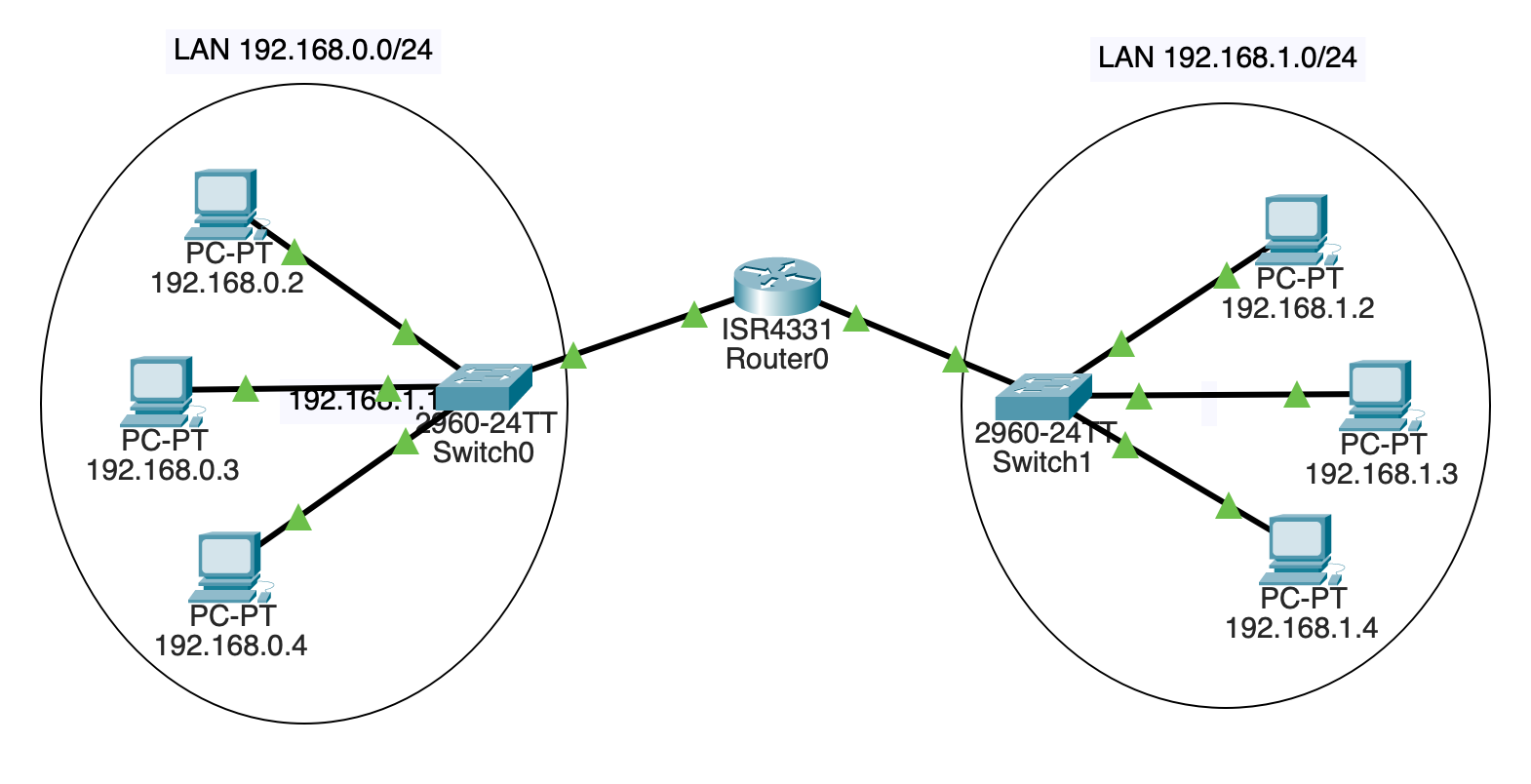
First of all, build two separate LANs. Each will have three PCs and a 2960 switch like before.
The left subnet will be 192.168.0.0/24. The right subnet will be 192.168.1.0/24.
Assign the left PCs the IP addresses on their FastEthernet0 interfaces:
192.168.0.2192.168.0.3192.168.0.4Assign the right PCs the IP addresses on their FastEthernet0 interfaces:
192.168.1.2192.168.1.3192.168.1.4All of them have subnet mask 255.255.255.0.
Connect the left PCs to one switch on any unused FastEthernet ports. Connect the right PCs to the other switch in the same way.
At this point, you should have two separate LANs.
Hit the fast-forward button if all the links aren’t green yet. If they stay red, something is wrong–double-check your settings.
For sanity, make sure 192.168.0.2 can ping the other two machines on its LAN. And make sure 192.168.1.3 can ping the other two machines on its LAN.
The router is going to route traffic between these two networks.
Click the “Network Devices” icon in the lower left. Then click “Routers” in the bottom left. Then drag a 4331 router in between the two.
This router is going to be connected to both switches. Each “side” of the router will have a different IP address.
We’re going to connect some wires here, but the link won’t come up yet. We’ll deal with that in a minute.
On the switch on LAN 192.168.0.0/24, use a Copper Straight-Through connector to connect the switch’s GigabitEthernet0/1 port to the router’s GigabitEthernet0/0/0 port.
On the switch on LAN 192.168.1.0/24, use the same type of connector to connect the switch’s GigabitEthernet0/1 port to the router’s GigabitEthernet0/0/1 port.
Note this is a different port on the router than the other switch is connected to! Both switches are plugged into different ports on the router.
We have the hardware in place now, but we don’t yet have any IP addresses assigned on the router. So let’s do that.
In the “Config” for the router, choose the GigabitEthernet0/0/0 interface and give it the IP address 192.168.0.1–it’s now part of the 192.168.0.0/24 subnet. While you’re here, click the “On” checkbox to power the port. This should bring up the connection and get you the green arrows.
Then go to the GigabitEthernet0/0/1 interface and give it the IP address 192.168.1.1–it’s now part of the 192.168.1.0/24 subnet. While you’re here, click the “On” checkbox to power the port.
Let’s try pinging the router. Go to any PC on the 192.168.0.0/24 LAN and trying pinging 192.168.0.1 (the router). It should reply.
Then go to any PC on the 192.168.1.0/24 subnet and try pinging 192.168.1.1. It should reply.
Now the ultimate test: get a console on PC 192.168.0.2 and try to ping 192.168.1.2 on the other subnet!
It… doesn’t work!
Why?
All the computers need to know two things:
We’ve put the subnet in, but not the default gateway.
For all the PCs on the 192.168.0.0/24 subnet, go into the “Config”, then choose the “Global” sidebar item. Enter 192.168.0.1 (the router!) in the “Default Gateway” field.
Do the same for all the PCs on the other subnet, except enter 192.168.1.1 as the default gateway.
Now you should be able to ping any PC from any other PC!
If you can’t, try pinging just on one LAN to make sure it works. And ping the router on that LAN to make sure that works.
In the last Packet Tracer project, we had a single router between two subnets. In this project, we’ll have multiple routers between subnets.
This complicates matters, because each router’s routing table needs to be edited so that it knows out which connection to forward packets.
In a larger LAN, a gateway protocol could be used to quickly distribute the information the routers needed.
But in our case, to keep it conceptually simple, we’ll just manually configure the routes in each of the three routers we’ll have.
FIVE subnets!
192.168.0.0/24192.168.1.0/24192.168.2.0/2410.0.0.0/1610.1.0.0/16And here’s a picture of it:
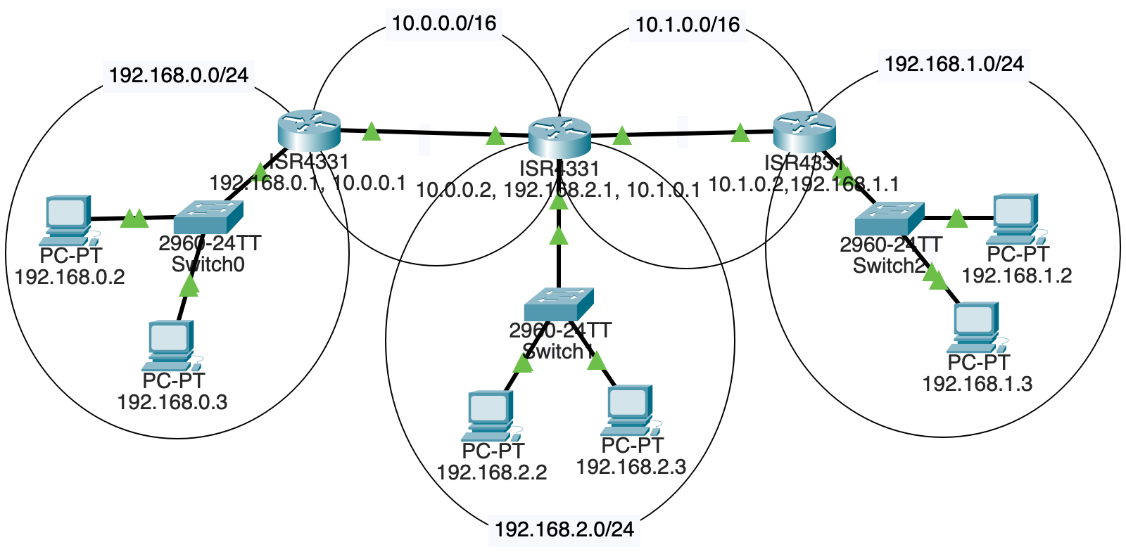
We’ll need:
Each LAN is connected to one router.
Two of the routers also connect to another router.
But, and this is the fun bit, the middle router is connected to two routers and another LAN!
Put straight-through copper connections between the components as shown in the diagram, above.
That router in the middle that connects to two other routers and a LAN? It doesn’t come with enough ports by default. We need to add one.
Luckily this is a virtual simulation, so you’re allowed to simulate virtual payment for the new components and won’t have to open your real wallet.
Select that router and go to the “Physical” tab.
Click “Zoom In” to get a better view.
The power switch is on the right side. Scroll over there and click it. (You can’t add components until you power it down.)
Two of the Ethernet connectors are in the upper left. Just right of those, there are two more ports that we can plug components into.
From the left sidebar, drag a “GLC-T” into the lower one of those ports (apparently it doesn’t work in the upper one), as shown below:
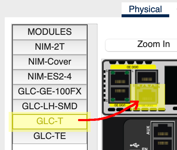
Then power the router back on.
Use these subnet numbers:
192.168.0.0/24192.168.1.0/24192.168.2.0/24By convention, routers often are the .1 on their subnet, e.g. 192.168.2.1. This isn’t a requirement.
Assign the 2 PCs and 1 of the routers IP addresses on the subnet. Connect them all to a switch.
Make sure the correct Ethernet port on the router has been set “On” in its config!
Sanity check: all computers on a subnet should be able to ping each other and their router.
Remember that when PCs send out traffic, they either know they’re sending it on the LAN (because the destination is on the same LAN), or they don’t know where the IP is. If they don’t recognize the IP as being on the same subnet, they send the traffic to their default gateway, i.e. the router that knows what to do with it.
Click on each PC in turn. Under “Config” in sidebar “Global/Settings”, set a static “Default Gateway” of that LAN’s router IP.
For example, if I’m on PC 192.168.1.2 and my router on that LAN is 192.168.1.1, I’ll set the PC’s default gateway to 192.168.1.1.
In fact, I’ll set the default gateway for all the PCs on the LAN to that value.
Do the same for the other two LANs.
In order to route properly, we need one subnet between the left and middle router, and another between the middle and right.
Use these subnets:
10.0.0.0/1610.1.0.0/16This means the left and right routers will have TWO IP addresses because they’re attached to two subnets.
But the middle router will have THREE IP addresses because it’s attached to three subnets! (i.e. attached to one LAN, and attached to two other routers.
Connect the subnets with copper straight-through connectors if you haven’t done so already..
We’re almost there, but if you’re on 192.168.0.2 and you try to ping 192.168.1.2, the traffic won’t get through.
This is because the router on subnet 192.168.0.0/24 doesn’t know where to send so that it arrives at 192.168.1.2.
We have to put that in.
We’re going to manually add “static routes” to each of the routers so that they know where to send things. As mentioned earlier, in real-life LANs, it would be more common to use gateway protocols to automatically get these routing tables set up.
But this is a lab–what would the fun be in that? (Actually it would be a very useful exercise, but this one is usefuller as an introduction.)
Let’s look at the network diagram again:
If a packet destined for 192.168.1.2 (on the right) leaves from 192.168.0.3 on the left, how does it get there?
We can see it must travel through all three routers. But when it arrives at the first one at 192.168.0.1 (the router for the LAN), where does that router send it?
Well, from there, we’ll head out on the 10.0.0.0/16 subnet to router 10.0.0.2.
So we have to add a route for the leftmost router saying, “Hey, if you get anything for subnet 192.168.0.0/24, forward it to 10.0.0.2 because that’s the next hop on the way.”
We do this by clicking on the leftmost router, then going to “Config”, and “Routing/Static” in the left sidebar.
The “Network” and “Mask” fields are the destination, and “Next Hop” is the router we should forward that traffic to.
In the case of the diagram, we’d add a route to the leftmost router like so (recalling that a \24 network has netmask 255.255.255.0):
Network:  192.168.1.0
Mask:     255.255.255.0
Next Hop: 10.0.0.2
And that gets us partway there! But, sadly and importantly, that middle router doesn’t know where to send traffic for 192.168.1.0/24, either.
So we have to add a route to that middle router that sends it on the next hop, but this time out its 10.1.0.0/16 interface:
Network:  192.168.1.0
Mask:     255.255.255.0
Next Hop: 10.1.0.2
And now we’re there! The router with IP 10.1.0.2 has an interface that is connected to 192.168.1.0/24. Our original packet is going to 192.168.1.2, and that’s on the same subnet! The router knows it can just send the traffic out on that interface.
Of course, that’s not all we have to do.
Add routing table entries for all the non-directly-connected subnets to each router.
Each router should have two static routing table entries so that all inbound and outbound traffic is covered.
If it’s all configured correctly, you should be able to ping any PC from any other PC! The routers forward the traffic to the other LANs!
In this chapter we’re taking a look at the select() function. This is a function that looks at a whole set of sockets and lets you know which ones have sent you data. That is, which ones are ready to call recv() on.
This enables us to wait for data on a large number of sockets at the same time.
Let’s say the server is connected to three clients. It wants to recv() data from whichever client sends it next.
But the server has no way of knowing which client will send data next.
In addition, when the server calls recv() on a socket with no data ready to read, the recv() call blocks, preventing anything else from running.
To block means that the process will stop executing here and goes to sleep until some condition is met. In the case of
recv(), the process goes to sleep until there’s some data to receive.
So we have this problem where if we do something like this:
data1 = s1.recv(4096)
data2 = s2.recv(4096)
data3 = s3.recv(4096)
but there’s no data ready on s1, then the process will block there and not call recv() on s2 or s3 even if there’s data to be received on those sockets.
We need a way to monitor s1, s2, and s3 at the same time, determine which of them have data ready to receive, and then call recv() only on those sockets.
The select() function does this. Calling select() on a set of sockets will block until one or more of those sockets is ready-to-read. And then it returns to you which sockets are ready and you can call recv() specifically on those.
select()First of all, you need the select module.
import selectIf you have a bunch of connected sockets you want to test for being ready to recv(), you can add those to a set() and pass that to select(). It will block until one is ready to read.
This set can be used as your canonical list of connected sockets. You need to keep track of them all somewhere, and this set is a good place. As you get new connections, you add them to the set, and as the connections hang up, you remove them from the set. In this way, it always holds the sockets of all the current connections.
Here’s an example. select() takes three arguments and return three values. We’ll just look at the first of each of these for now, ignoring the other ones.
read_set = {s1, s2, s3}

ready_to_read, _, _ = select.select(read_set, {}, {})
At this point, we can go through the sockets that are ready and receive data.
for s in ready_to_read:
data = s.recv(4096)select() with Listening SocketsIf you’ve been looking closely, you might have the following question: if the server is blocked on a select() call waiting for incoming data, how can it also call accept() to accept incoming connections? Won’t the incoming connections have to wait? Furthermore, accept() blocks… how will we get back to the select() if we’re blocked on that?
Fortunately, select() provides us with an answer: you can add a listening socket to the set! When the listening socket shows up as “ready-to-read”, it means there’s a new incoming connection to accept().
Putting it all together, we get the core of any main loop that uses select():
add the listener socket to the set

main loop:

    call select() and get the sockets that are ready to read

    for all sockets that are ready to read:

        if the socket is the listener socket:
            accept() a new connection
            add the new socket to our set!

        else the socket is a regular socket:
            recv() the data from the socket

            if you receive zero bytes
                the client hung up
remove the socket from tbe set!select()?select() actually takes three arguments. (Though for this project we only need to use the first one, so this section is purely informational.)
They correspond to:
And the return values map to these, as well.
read, write, exc = select.select(read_set, write_set, exc_set)But again, for this project, we just use the first and ignore the rest.
read, _, _ = select.select(read_set, {}, {})I told a bit of a lie. There’s an optional fourth arguments, the timeout. It’s a floating point number of seconds to wait for an event to occur; if nothing occurs in that timeframe, select() returns and none of the returned sockets are shown as ready.
You can also specify a timeout of 0 if you want to just poll the sockets.
select() with send()If your computer tries to send too much too fast, the call to send() might block. That is, the OS will have it sleep while it processes the backlog of data to be sent.
But let’s say you really don’t want to have the call block and want to keep processing.
You can query with select() to make sure a socket won’t block with a send() call by passing a set containing the socket descriptor as the second argument.
And it’ll work in much the same way as the “ready to read” set works, above.
Why can’t we just call recv() on all the connected sockets? What does select() buy us?
When select() shows a socket “ready-to-read”, what does it mean if the socket is a listening socket versus a non-listening socket?
Why do we have to add the listener socket to the set, anyway? Why not just call accept() and then call select()?
In this project we’re going to write a server that uses select() to handle multiple simultaneous connections.
The client is already provided. You fill in the server.
Grab this ZIP file15 with all the input files.
The select_client.py file is already complete.
You have to fill in the select_server.py file to get it going.
Your server should do the following:
When a client connects, the server prints out the client connection info in this form (it’s the client IP and port number in front):
('127.0.0.1', 61457): connectedWhen a client disconnects, the server prints out the late client’s connection info in this form:
('127.0.0.1', 61457): disconnectedHint: You can use the .getpeername() method on a socket to get the address of the remote side even after it has disconnected. It’ll come back as a tuple containing ("host", port), just like what you pass to connect().
When a client sends data, the server should print out the length of the data as well as the raw bytestring object received:
('127.0.0.1', 61457) 22 bytes: b'test1: xajrxttphhlwmjf'Running the server:
python select_server.py 3490Running the clients:
python select_client.py alice localhost 3490
python select_client.py bob localhost 3490
python select_client.py chris localhost 3490
The first argument to the client can be any string–the server prints it out with the data to help you identify which client it came from.
Example output:
waiting for connections
('127.0.0.1', 61457): connected
('127.0.0.1', 61457) 22 bytes: b'test1: xajrxttphhlwmjf'
('127.0.0.1', 61457) 22 bytes: b'test1: geqtgopbayogenz'
('127.0.0.1', 61457) 23 bytes: b'test1: jquijcatyhvfpydn'
('127.0.0.1', 61457) 23 bytes: b'test1: qbavdzfihualuxzu'
('127.0.0.1', 61457) 24 bytes: b'test1: dyqmzawthxjpkgpcg'
('127.0.0.1', 61457) 23 bytes: b'test1: mhxebjpmsmjsycmj'
('127.0.0.1', 61458): connected
('127.0.0.1', 61458) 23 bytes: b'test2: bejnrwxftgzcgdyg'
('127.0.0.1', 61457) 24 bytes: b'test1: ptcavvhroihmgdfyw'
('127.0.0.1', 61458) 24 bytes: b'test2: qrumcrmqxauwtcuaj'
('127.0.0.1', 61457) 26 bytes: b'test1: tzoitpusjaxljkfxfvw'
('127.0.0.1', 61457) 17 bytes: b'test1: mtcwokwquc'
('127.0.0.1', 61458) 18 bytes: b'test2: whvqnzgtaem'
('127.0.0.1', 61457): disconnected
('127.0.0.1', 61458) 21 bytes: b'test2: raqlvexhimxfgl'
('127.0.0.1', 61458): disconnectedWe’ve learned that IP is responsible for routing traffic around the Internet. We’ve also learned that it does it with IP addresses, which we commonly show in dots-and-numbers format for IPv4, such as 10.1.2.3.
But as humans, we rarely use IP addresses. When you use your web browser, you don’t typically put an IP address in the address bar.
Even in our projects, we tended to type localhost instead of our localhost address of 127.0.0.1.
The general process for converting a name like www.example.com that humans use into an IP address that computers use is called domain name resolution, and is provided by a distributed group of servers that comprise the Domain Name System, or DNS.
From a user standpoint, we configure our devices to have a “name server” that they contact to convert those names to IP addresses. (Probably this is configured with DHCP, but more on that later.)
When you try to connect to example.com, your computer contacts that name server to get the IP address.
If that name server knows the answer, it supplies it. But if it doesn’t, then a whole bunch of wheels get put into motion.
Let’s start diving down into that process.
If haven’t ever registered a domain (such as example.com or oregonstate.edu or google.com or army.mil), the process is something like this:
But doing this is completely disconnected from the idea of an IP address. Indeed, domains can exist without IP addresses–they just can’t be used.
Once you have your domain, you can contact a hosting company that will provide you with an IP address on a server that you can use.
Now you have the two pieces: the domain and the IP address.
But you still have to connect them so people can look up your IP if they have your domain name.
To do this, you add a database record with the pertinent information to a server that’s part of the DNS landscape: a domain name server.
Usually called name servers for short, these servers contain IP records for the domain in which they are an authority. That is, a name server doesn’t have records for the entire world; it just has them for a particular domain or subdomain.
A subdomain is a domain administered by the owner of a domain. For example, the owner of
example.commight make subdomainssub1.example.comandsub2.example.com. These aren’t hosts in this case–but they can have their own hosts, e.g.host1.sub1.example.com,host2.sub1.example.com,somecompy.sub2.example.com.Domain owners can make as many subdomains as they want. They just have to make sure they have a name server set up to handle them.
A name server that’s authoritative for a specific domain can be asked about any host on that domain.
The host is often the first “word” of a domain name, though it’s not necessarily.
For example with www.example.com, the host is a computer called www on a domain example.com.
A single name server might be authoritative for many domains.
But even if a name server doesn’t know the IP address of the domain it’s been asked to provide, it can contact some other name servers to figure it out. From a user perspective, this process is transparent.
So, easy-peasy. If I don’t know the domain in question, I’ll just contact the name server for that domain and get the answer from them, right?
We have an issue, though. How can I connect to the name server for a domain if I don’t know what the name server is for a domain?
To solve this, we have a number of root name servers that can help us on our way. When we don’t know an IP, we can start with them and ask them to tell us the IP, or tell us which other server to ask. More on that process in a minute.
Computers are preconfigured with the IP addresses of the 13 root name servers. These IPs rarely ever change, and only one of them is needed to work. Computers that perform DNS frequently retrieve the list to keep it up to date.
The root name servers themselves are named a to m:
a.root-servers.net
b.root-servers.net
c.root-servers.net
...
k.root-servers.net
l.root-servers.net
m.root-servers.netLet’s start by doing a query on a computer called www.example.com. We need to know its IP address. We don’t know which name server is responsible for the example.com domain. All we know is our list of root name servers.
Let’s choose a random root server, say c.root-servers.net. We’ll contact it and say, “Hey, we’re looking for www.example.com. Can you help us?”
But the root name server doesn’t know that. It says, “I don’t know about that, but I can tell you if you’re looking for any .com domain, you can contact any one of these name servers.” It attaches a list of name servers who know about the .com domains:
a.gtld-servers.net
b.gtld-servers.net
c.gtld-servers.net
d.gtld-servers.net
e.gtld-servers.net
f.gtld-servers.net
g.gtld-servers.net
h.gtld-servers.net
i.gtld-servers.net
j.gtld-servers.net
k.gtld-servers.net
l.gtld-servers.net
m.gtld-servers.net
So we choose one of the .com name servers.
“Hey h.gtld-servers.net, we’re looking for www.example.com. Can you help us?”
And it answers, “I don’t know that name, but I do know the name servers for example.com. You can talk to one of them. It attaches the list of name servers who know about the example.com domain:
a.iana-servers.net
b.iana-servers.net
So we choose one of those servers.
“Hey a.iana-servers.net, we’re looking for www.example.com. Can you help us?”
And that name server answers, “Yes, I can! I know that name! Its IP address is 93.184.216.34!”
So for any lookup, we start with root name server and it directs us on where to go to find more info. (Unless the information has been cached somewhere, but more on that later.)
The Domain Name System is split into logical administrative zones. A zone is, loosely, a collection of domains under the authority of a particular name server.
But that’s an oversimplification. There could be one or more domains in the same zone. And there could be a number of name servers working in that same zone.
Think of the zones as all the domains and subdomains some administration is responsible for.
For example, in the root zone, we saw there were a number of name servers responsible for that lookup. And also in the .com zone, there were a number of different name servers there with authority.
When you write software that uses domain names, it calls a library to do the DNS lookup. You might have noticed that in Python when you called:
s.connect(("example.com", 80))you didn’t have to worry about DNS at all. Behind the scenes, Python did all that work of looking up that domain in DNS.
In C, there’s a function called getaddrinfo() that does the same thing.
The short of it is that there’s a library that we can use and we don’t have to write all that code ourselves.
The OS also has a record containing its default name server to use for lookups. (This is sometimes configured by hand, but more commonly is configured through DHCP.) So when you request a lookup, your computer first goes to this server.
But wait a minute–how does that tie into the whole root server hierarchy thing?
The answer: caching!
Imagine all the DNS lookups that are happening globally. If we had to go to the root servers for every request, not only would that take a long time for repeated requests, but the root servers would get absolutely hammered.
To avoid this, all DNS resolver libraries and DNS servers cache their results.
As it is, the root servers handle literally trillions of requests per day.
This way we can avoid overloading the root servers with repeated requests.
So we’re going to have to amend the outline we already went over.
Ask our resolver library for the IP address. If it has it cached, it will return it.
If it doesn’t have it, ask our local name server for the IP address. If it has it cached, it will return it.
If it’s not cached and if this name server has another upstream name server (that is, another nameserver it can appeal to for answers), it asks that name server for the answer.
If it’s not cached and if this name server does not have another upstream name server, it goes to the root servers and the process continues as before.
With all these possible opportunities to get a cached result, it really helps take the load off the root name servers./
Lots of WiFi routers you get also run caching name servers. So when DHCP configures your computer, your computer uses your router as a DNS server for the computers on your LAN. This gives you a snappy response for DNS lookups since you have a really short ping time to your router.
Since the IP address for a domain or host might change, we have to have a way to expire cache entries.
This is done through a field in the DNS record called time to live (TTL). This is the number of seconds a server should cache the results. It’s commonly set to 86400 seconds (1 day), but could be more or less depending on how often a zone administrator thinks an IP address will change.
When a cache entry expires, the name server will have to once again ask for the data from upstream or the root servers if someone requests it.
So far, we’ve talked about using DNS to map a host or domain name to an IP address. This is one of the types of records stored for a domain on a DNS server.
The common record types are:
A: An address record for IPv4. This is the type of record we’ve been talking about this whole time. Answers the question, “What is the IPv4 address for this host or domain?”
AAAA: An address record for IPv6. Answers the question, “What is the IPv6 address for this host or domain?”
NS: A name server record for a particular domain. Answers the question, “What are the name servers answering for this host or domain?”
MX: A mail exchange record. Answers the question, “What computers are responsible for handling mail on this domain?”
TXT: A text record. Holds free-form text information. Is sometimes used for anti-spam purposes and proof-of-ownership of a domain.
CNAME: A canonical name record. Think of this as an alias. Makes the statement, “Domain xyz.example.com is an alias for abc.example.com.”
SOA: A start of authority record. This contains information about a domain, including its main name server and contact information.
There are a lot of DNS record types.
Typical users of the Internet don’t have a static IP address (that is, dedicated or unchanging) at their house. If they reboot their modem, their ISP might hand them a different IP address.
This causes a ruckus with DNS because any DNS records pointing to their public IPs would be out of date.
Dynamic DNS (DDNS) aims to solve this problem.
In a nutshell, there are two mechanisms at play:
A way for a client to tell the DDNS server what their IP address is.
A very short TTL on the DDNS server for that record.
While DNS defines a way to send update records, a common other way is for a computer on your LAN to periodically (e.g. every 10 minutes) contact the DDNS provider with an authenticated HTTP request. The DDNS server will see the IP address it came from and use that to update its record.
What if you have a dots-and-numbers IP address and want the host name for that IP? You can do a reverse DNS lookup.
Note that not all IP addresses have such records, and often a reverse DNS query will come up empty.
What is your name server for your computer right now? Search the net for how to look it up on your particular OS.
Do the root name servers know every IP address in the world?
Why would anyone use dynamic DNS?
What is TTL used for?
In this chapter we’ll be taking a look at network address translation, or NAT.
This is a service provided on a router which hides a “private” LAN from the rest of the world.
The router acts as a middleman, translating internal IP addresses to a single external IP address. It keeps a table of these connections so when packets arrive on either interface, the router can rewrite them appropriately.
We say the LAN behind the NAT router is a “private network”, and the external IP address the router presents for that LAN is the “public IP”.
Imagine how an anonymous snail-mail program might work.
You write a letter addressed to the recipient with your return address on it.
Instead of mailing it directly, you hand the letter to an anonymizer. The anonymizer removes your letter from the envelope and puts it in another envelope with the same recipient, but replaces the return address with the anonymnizer’s address. It also records that this sender wrote a letter to this recipient.
The recipient gets the letter. All they see is the anonymizer’s return address on the letter.
The recipient responds to the letter, and sends the response back to the anonymizer. The recipient lists themselves as the return address.
The anonymizer receives the mail and notes it’s from the recipient. It looks in its records to determine the person who originally sent a message to the recipient.
The anonymizer takes the response out of the envelope and puts it in a new envelope with the destination address being the original sender, and the return address remaining the original recipient.
The original sender receives the response.
Note that the original recipient never knew the original sender’s address; they only knew the anonymizer’s address.
NAT is very, very common. It almost certainly runs on every IPv4 LAN.
But why?
There are two main reasons to use this type of service.
You want to hide your network details from the rest of the world.
You need more IP addresses than either (a) anyone is willing to allocate to you or (b) you’re willing to pay for.
There’s no easy way to get random, unsolicited packets onto the private network through the gateway running NAT.
You can possibly do it with something called source routing, but that’s not commonly enabled by ISPs.
You’d have to have the private IP on the packet and get that packet to the router. There’s no way to do this unless you’re on the same LAN as the router, and that’s really unlikely.
Regarding the second point, we should talk about the phenomenon known as address space exhaustion.
There are really a limited number of IPv4 addresses in the world. As such, getting a large block of them costs a lot of money.
It’s a lot cheaper to get just a handful of addresses (e.g. a /20 or /24 or /4 network) and then have large private networks behind NAT routers. This way you can have a lot of IPs, but they all present to the world as coming from the single public IP.
This is really the motivation behind using NAT everywhere. There was a time when we were genuinely about to run out of IPv4 addresses, and NAT saved us.
There are subnets that are reserved for use as private networks. Routers don’t forward these addresses directly. If a router on the greater Internet sees an IP from one of these subnets, it will drop it.
For IPv4 there are three such subnets:
10.0.0.0/8172.16.0.0/12192.168.0.0/16The last of these is really common on household LANs.
Again, routers on the Internet will drop packets with these addresses. The only way data gets from these IPs onto the Internet is via NAT.
For this demo, we’re going to use IP:port notation. The number after the colon is the port number.
Also, we’ll use the term “Local Computer” to refer to the computer on the LAN, and “Remote Computer” or “Remote Server” to refer to the distant computer it’s connecting to.
And finally, the local LAN router will just be called “The Router” or the “NAT Router”.
Let’s go!
On my LAN, I want to go from 192.168.1.2:1234 on my private LAN to the public address 203.0.113.24:80–that’s port 80, the HTTP server.
The first thing my computer does is check to see if the destination IP address is on my LAN… Since my LAN is 192.168.0.0/16 or smaller, then no, it’s not.
So my computer sends it to the default gateway, my router that has NAT enabled.
The router is going to play the role of the “anonymizer” middleman in the earlier analogy example. And recall that the router has two interfaces on it–one faces the internal 192.168.0.0/16 private LAN, and the other faces the greater Internet with a public, external IP. Let’s use 192.168.1.1 as the private IP address on the router and 198.51.100.99 as the public IP.
So the LAN looks like this:
+----------+-------------+
|  Local   |             |
| Computer | 192.168.1.2 |>-------+
+----------+-------------+        |
                                  |
                                  ^
                          +---------------+
                          |  192.168.1.1  |  Internal IP
                          +---------------+
                          |    Router     |  NAT-enabled
                          +---------------+
                          | 198.51.100.99 |  External IP
                          +---------------+
                                  v
                                  |
                                  |
                       {The Greater Internet}
The router now has to “repackage” the data for the greater Internet. This means rewriting the packet source to be from the router’s public IP and some unused port on the public interface of the router. (The port doesn’t need to be the same as the port originally on the packet. The router allocates a random unused port when the new packet is sent out.))
So the router records all this information:
| Computer | IP | Port | Protocol |
|---|---|---|---|
| Local Private Address | 192.168.1.2 | 1234 | TCP |
| Remote Public Address | 203.0.113.24 | 80 | TCP |
| Router Public Address | 198.51.100.99 | 5678 | TCP |
(Note: except for 80, since we’re connecting to HTTP in this example, all port numbers were randomly chosen.)
So while the original packet was:
192.168.1.2:1234 --> 203.0.113.24:80

     Local               Remote
    Computer            Computer
the NAT router rewrites it to be the same destination, but the router as the source.
198.51.100.99:5678 --> 203.0.113.24:80

    NAT router             Remote
                          Computer
From the destination’s point of view, it is completely unaware that this isn’t originally from the router itself.
So the destination replies with some HTTP data, sending it back to the router:
203.0.113.24:80 --> 198.51.100.99:5678

    Remote              NAT router
   Computer
The router then looks at its records. It says, “Wait a moment–if I get data on port 5678, that means I need to translate this back to a private IP on the LAN!
So it translates the message so that it’s no longer addressed to the router, but instead is sent to the private source IP recorded earlier:
203.0.113.24:80 --> 192.168.1.2:1234

    Remote               Local
   Computer             Computer
And sends that out on the LAN. And its received! The LAN computer thinks it’s talking to the remote server, and the remote server thinks it’s talking to the router! NAT!
It might be a little confusing in that last step that the packet is coming from the NAT router but is actually IP addressed like it came from the Remote Computer. This is OK on the LAN because the NAT router sends that IP packet out with an Ethernet address of the Local Computer on the LAN. Or, put another way, the NAT router can use link layer addressing to get the packet delivered to the Local Computer and the IP address of where that packet came from doesn’t have to match the internet IP of the NAT router.
Since IPv6 has tons of addresses, do we really need NAT? And the technical answer is “no”. Part of the reason IPv6 came about was to get rid of this nasty NAT middleman business.
That said, there is a reserved IPv6 subnet for private networks:
fd00::/8There’s some additional structure in the “host” portion of the address, but you can read about it on Wikipedia if you want.
Like the IPv4 private subnets, IP addresses from this subnet are dropped by routers on the greater Internet.
NAT doesn’t work for IPv6, but there is another way to do the translation with network prefix translation.
But what about the whole idea that people can’t easily get unsolicited packets onto your LAN? Well, you’re just going to have to configure your firewall properly to keep people out. But that’s a story for another time.
If you have a server running behind the NAT router, how can it serve content to the outside world? After all, no one on the outside can refer to it by its internal IP address–all they can see is the router’s external IP.
But you can configure the NAT router to do something called port forwarding.
For example, you could tell it that traffic sent to its public IP port 80 should be forwarded to some private IP on port 80. The router forwards the traffic, and the original sender is unaware that its traffic is ultimately arriving at a private IP.
There’s no reason the same port must be used.
For example, SSH uses port 22, and that’s fine on the computer on the private network. But if you forward from the public port 22, you’ll find malicious actors are continuously trying to log in through it. (Yes, even on your computer at home.) So it’s more common to use some other uncommon port as the public SSH port, and then forward it to port 22 on the LAN.
Look up your computer’s internal IP address. (Might have to search the net to see how to do this.) Then go to google.com and type “what is my ip”. The numbers are (very probably) different. Why?
What problems does NAT solve?
When you first open your laptop at the coffee shop, it doesn’t have an IP address. It doesn’t even know what IP address it should have. Or what its name servers are. Or what its subnet mask is.
Of course, you could manually configure it! Just type in the numbers that the cashier hands you with your coffee!
OK, that doesn’t happen. No one would bother. Or they’d use a duplicate address. And things wouldn’t work. And they’d probably rage-drink their coffee and never return.
It would be better if there were a way to automatically configure a computer that just arrived on the network, wouldn’t it?
That’s what the Dynamic Host Configuration Protocol (DHCP) is for.
The overview:
Client --> [DHCPDISCOVER packet] --> Server

Client <-- [DHCPOFFER packet] <-- Server

Client --> [DHCPREQUEST packet] --> Server

Client <-- [DHCPACK packet] <-- Server
The details:
When your laptop first tries to connect to the network, it sends a DHCPDISCOVER packet to the broadcast address (255.255.255.255) over UDP to port 67, the DHCP server port.
Recall that the broadcast address only propagates on the LAN–the default gateway does not forward it.
On the LAN is another computer acting as the DHCP server. There’s a process running on it waiting on port 67.
The DHCP server process sees the DISCOVER and decides what to do with it.
The typical use is that the client wants an IP address. We call this leasing an IP from the DHCP server. The DHCP server is tracking which IPs have been allocated and which are free out of its pool.
In response to the DHCPDISCOVER packet, the DHCP server sends a DHCPOFFER response back to the client on port 68.
The offer contains an IP address and potentially a lot of other pieces of information including, but not limited to:
The client can accept or ignore the offer. (Maybe there are multiple DHCP servers making offers, but the client may only accept one of them.)
If the offer is accepted, the client sends a DHCPREQUEST back to the server notifying it that it wants that particular IP address.
Finally, if all’s well, the server replies with an acknowledgment packet, DHCPACK.
At that point, the client has all the information it needs to participate on the network.
Reflect on the advantages of using something like DHCP over manually configuring the devices on your LAN.
What types of information does a DHCP client receive from the DHCP server?
The dig utility is a great command line tool for getting DNS information from your default name server, or from any name server.
On Macs:
brew install bindOn WSL:
sudo apt install dnsutilsType:
dig example.comand see what it gives back.
; <<>> DiG 9.10.6 <<>> example.com
;; global options: +cmd
;; Got answer:
;; ->>HEADER<<- opcode: QUERY, status: NOERROR, id: 60465
;; flags: qr rd ra ad; QUERY: 1, ANSWER: 1, AUTHORITY: 0, ADDITIONAL: 1

;; OPT PSEUDOSECTION:
; EDNS: version: 0, flags:; udp: 1232
;; QUESTION SECTION:
;example.com.                   IN      A

;; ANSWER SECTION:
example.com.            79753   IN      A       93.184.216.34

;; Query time: 23 msec
;; SERVER: 1.1.1.1#53(1.1.1.1)
;; WHEN: Fri Nov 18 18:37:13 PST 2022
;; MSG SIZE  rcvd: 56
That’s a lot of stuff. But let’s look at these lines:
;; ANSWER SECTION:
example.com.            79753   IN      A       93.184.216.34
That’s the IP address for example.com! Notice the A? That means this is an address record.
You can get other record types, as well. What if you want the mail exchange server for oregonstate.edu? You can put that on the command line:
dig mx oregonstate.eduWe get:
;; ANSWER SECTION:
oregonstate.edu. 600 IN MX 5 oregonstate-edu.mail.protection.outlook.com.
Or if we want the name servers for example.com, we can:
dig ns example.comIf you dig an A record, you’ll see a number on the line:
;; ANSWER SECTION:
example.com.            78236   IN      A       93.184.216.34
In this case, it’s 78236. This is the TTL of an entry in the cache. This is telling you that the name server you used has cached that IP address, and it won’t expire that cache entry until 78,236 more seconds have elapsed. (For reference, there are 86,400 seconds in a day.)
If you get an entry that’s cached in your name server, you’ll see AUTHORITY: 0 in the dig output:
;; flags: qr rd ra ad; QUERY: 1, ANSWER: 1, AUTHORITY: 0, ADDITIONAL: 1
                                            ^^^^^^^^^^^^
But if the entry comes directly from the name server that’s responsible for the domain, you’ll see AUTHORITY: 1 (or some positive number).
Just type dig and hit return and you’ll see all the root DNS servers, probably both their IPv4 (record type A) and IPv6 (record type AAAA) addresses
If you know a name server that you want to query, you can use an @ sign to specify that server.
Two popular free-to-use name servers are 1.1.1.1 and 8.8.8.8.
Let’s ask one of them for the IP of example.com
dig @8.8.8.8 example.comAnd we get our expected answer. (Though the TTL is probably different–these are different servers and their cache entries have different ages, after all.)
There were a bunch of root name servers, so let’s dig example.com at one of them:
dig @l.root-servers.net example.comWe get some interesting results:
com.                    172800  IN      NS      a.gtld-servers.net.
com.                    172800  IN      NS      b.gtld-servers.net.
com.                    172800  IN      NS      c.gtld-servers.net.
com.                    172800  IN      NS      d.gtld-servers.net.
and then some.
That’s not example.com… and look–those are NS records, name servers.
This is the root server telling us, “I don’t know who example.com is, but here are some name servers that know what .com is.”
So we choose one of those and dig there:
dig @c.gtld-servers.net example.comAnd we get:
example.com.            172800  IN      NS      a.iana-servers.net.
example.com.            172800  IN      NS      b.iana-servers.net.
Same thing again, more NS name server records. This is the c.gtld-servers.net name server telling us, I don’t know the IP for example.com, but here are some name servers that might!”
So we try again:
dig @a.iana-servers.net example.comAnd at last we get the A record with the IP!
example.com. 86400 IN A 93.184.216.34You can also use +trace on the command line to watch the entire query from start to end:
dig +trace example.comTry to answer the following:
What’s the IP address of microsoft.com?
What’s the mail exchange for google.com?
What are the name servers for duckduckgo.com?
Following the process in the Digging from a Root Name Server in the section above, start with a root name server and dig your way down to www.yahoo.com (NOT yahoo.com).
Note that this ends in a CNAME record! You’ll have to repeat the process with the alias named by the CNAME record starting from the root servers again.
Add to your document the dig commands you used to get the IP address. Each dig command should be @ a different name server, starting with the root.
A NOTE ON LEGALITY: It’s unclear whether or not it is legal to portscan a computer you do not own. We’ll be doing all our portscanning on localhost. Don’t portscan computers you do not have permission to!
A port scan is a method of determining which ports on a computer a ready to accept connections. In other words, which ports have a server listening on them.
The port scan is often the first line of attack on a system. Before being able to connect to see if some vulnerabilities can be found in any listening servers, we need to know which servers are running in the first place.
A portscanner will attempt to find listening server processes on a range of ports on a specified IP. (Sometimes the range is all ports.)
With TCP, the general approach is to try to set up a connection with the connect() call on the candidate port. If it works, we have an open port, and the portscanner outputs that information. Nothing is sent over the connection, and it is closed immediately.
The job of the portscanner is to identify open ports, not to send or receive other data unnecessarily.
Calling connect() causes the TCP connection to complete its three-way handshake. This isn’t strictly necessary, since if the portscanner gets any reply from the server (i.e. the second part of the three way handshake) then we know the port is open. Completing the handshake would cause the remote OS to wake up the server on that port for a connection we know we’re just going to close anyway.
Some TCP portscanners will instead build a TCP SYN packet to start the handshake and send that to the port. If they get a SYN-ACK reply, they know the port is open. But then, instead of completing the handshake with an ACK, they send a RST (reset) causing the remote OS to terminate the nascent connection entirely–and causing it to not wake up the server on that port.
You can write software that builds custom TCP packets with raw sockets. Usually you need to be a superuser/admin to use these.
Since there is no connection with UDP, port scans are a little less exact.
One technique is to send a UDP packet to a port and see if you get an ICMP “destination unreachable” message back. If so, the port is not open.
If you don’t get a response, maybe the port is open. Or maybe the UDP packet is being filtered out and dropped with no ICMP response.
Another option is to send a UDP packet to a known port that might have a server behind it. If you get a response from the server, you know the port is open. If not, it’s closed or your traffic was filtered out.
Why shouldn’t you portscan random computers on the Internet?
What’s the purpose of using a portscanner?
A favorite component of every bad hacker movie ever is the firewall. It’s clear from those bad movies that it has something to do with security, but the exact role is ambiguous; it’s only apparent that a bad guy getting through the firewall is a bad thing.
But back to reality: a firewall is a computer (often a router) that restricts certain types of traffic between one interface and another. So instead of forwarding every packet of every type from every port, it might decide to drop those packets instead.
The upshot is that if someone in trying to connect to a port on the far side of a firewall, the firewall might prevent that connection depending on how it is configured.
In this chapter, we’ll be speaking conceptually about firewalls, but won’t get into any specifics about practical configuration. There are many implementations of firewalls out there, and they all tend to have different methods of configuration.
If you think about a packet arriving at a router, that router has the capability to inspect that packet all it wants. It can look at the source and destination IPs, or the ports, or even the application layer data.
So that gives it the opportunity to make a decision about whether or not to keep forwarding that packet based on any of that data.
For example, the firewall might be configured to allow any port 80 (HTTP) traffic to come from the outside of the firewall to the inside, but block incoming traffic on all other destination ports.
Or maybe it’ll be configured to only allow certain IP addresses to connect.
So the firewall, on receipt of a packet, looks at its configured rules and decides whether or not to drop the packet (if it’s being filtered out), or forward the packet normally.
When it decides to drop the packet, it has a more options. It can either silently drop it, or it can reply with a ICMP “destination unreachable” message.
That basic filtering gives some a control, but there are still some things you might want to do that it can’t manage.
For example, if someone behind the firewall establishes a TCP connection over the Internet from a random port, we want to be able to get traffic back to that host from that random port.
With plain filtering, we’d just have to allow traffic on all those ports.
But with stateful filtering, the firewall tracks the state of TCP connections that have been initiated from behind the firewall. The firewall sees the TCP three-way handshake and knows then that there is a valid connection. It can then safely allow traffic back that’s destined for the inside computer’s random port number.
Stateful filtering is also used with UDP traffic, even though it’s connectionless. The firewall sees a UDP packet go out, and it’ll allow incoming UDP packets to that port. (For a while. Since it’s connectionless, there’s no way to tell when the server and client and done. So the firewall will timeout UDP rules after they haven’t been used for a while.)
In order to keep the firewall from timing-out on any of its rules, the programs can send keepalive messages. TCP actually has a specific message type for this, and the OS will periodically send empty
ACKpackets out to keep anyone from timing out. (If programming with sockets, you will likely need to set theSO_KEEPALIVEoption.)The keepalive can also be effectively implemented by a program using UDP, as well. It could be configured to send a custom keepalive packet to the receiver (who would reply with some kind of ACK) every so often.
Keepalive is only an issue for programs that have long periods of no network traffic.
Finally, filtering could also be done at the application layer. If the firewall digs deeply enough into the packet, it might see that it’s HTTP or FTP data, for example. With that knowledge, it could allow or deny all HTTP traffic, even if it’s arriving on a non-standard port.
In a home network, it’s really common for the firewall to also be the router and the switch and do NAT.
It’s all rolled into one.
But there’s nothing stopping us from having a separate firewall computer on the network that only decides whether or not to allow traffic.
And there’s no rule that one side of the firewall must be a private network and the other side a public network. Both sides could be private networks or public networks, or one private and one public.
The role of the firewall at its core is not to separate public and private networks–that’s NAT’s role–but rather to control which traffic is allowed to pass through the firewall.
You can also set up a firewall just on your computer (and this is commonly done). Typically this is set up to allow all connections from the computer going out, but to restrict connections from other computers coming in.
In MacOS and Windows, the firewall is something that can simply be turned on and then it will start blocking traffic based on some common rules.
If you need some specific ports unblocked, you’ll have to manually add those.
Linux has firewall support through a mechanism called iptables. This isn’t the most straightforward thing to configure, but it’s powerful enough to build a NAT router/firewall from scratch.
What’s the difference/relationship between a firewall and a router?
What’s the difference/relationship between a firewall and NAT?
What’s the funniest or most painful thing in this NCIS clip?
“You won’t know who to trust…”
—Gregor Ivanovich, Sneakers
When your server receives data from someone on the Internet, it’s not good enough to trust that they have good intentions.
There are lots of bad actors out there. You have to take steps to prevent them from sending things that crash your server processes or, worse, give them access to your server machine itself.
In this chapter we’re going to take a high-level look at some issues that might arise from users trying to send malicious data.
The two big ideas here are:
Think like a villain. What could someone pass your code that would crash it or make it behave in an unexpected way?
Don’t trust anything from the remote side. Don’t trust that it will be a reasonable length. Don’t trust that it will contain reasonable data.
This is something that mostly affects memory-unsafe languages like C or C++.
The idea is:
Your program allocates a fixed size region of memory to use.
Your program reads some data into that memory region over a network connection.
The attacker sends more data than can fit in that memory region. This data is carefully constructed to contain a payload.
Your program, without thinking about it, writes the data from the attacker, filling the memory region and overflowing into whatever is in memory after that.
Depending on how things are written, the attacker could overwrite the return address value on the stack, causing the function to return into the attacker’s payload and run that. The payload manipulates the system to install a virus or change the system to otherwise allow remote access.
Modern OSes try to mitigate by making the stack and heap regions of memory non-executable, and the code region of memory non-writable.
As a developer, you need to write code in C that properly performs bounds-checking and never writes to memory it doesn’t intend to.
These attacks are ones where you build a command using some data the user has provided to you. And then run that command.
A malicious user can feed you data that causes another command to be run.
In many languages, there’s a feature that allows you to run a command via the shell.
For example, in Python you can run the ls command to get a directory listing like this:
import os

os.system("ls")
Let’s say you write a server that receives some data from a user. The user will send 1, 2 or 3 as data, depending on the function they want to select.
You run some code in your server like this:
os.system("mycommand " + user_input)So if the user sends 2, it will run mycommand 2 as expected and return the output to the user.
To be safe, the mycommand program verifies that the only allowable inputs are 1, 2, or 3 and returns an error if something else is passed.
Are we safe?
No. Do you see how?
The user could pass the input:
1; cat /etc/passwdThis would cause the following to be executed:
mycommand 1; cat /etc/passwdThe semicolon is the command separator in bash. This causes the mycommand program to execute, followed by a command that shows the contents of the Unix password file.
To be safe, all the special characters in the input need to be stripped or escaped so that the shell doesn’t interpret them.
There’s a similar attack called SQL Injection, where a non-carefully crafted SQL query can allow a malicious user to execute arbitrary SQL queries.
Let’s say you build a SQL query in Python like this, where we get the variable username over the network in some way:
q = f"SELECT * FROM users WHERE name = '{username}'So if I enter Alice for the user, we get the following perfectly valid query:
SELECT * FROM users WHERE name = 'Alice'And then I run it, no problem.
But let’s think like a villain.
What if we entered this:
Alice' or 1=1 --Now we get this:
SELECT * FROM users WHERE name = 'Alice' or 1=1 -- 'The -- is a comment delimiter in SQL. Now we’ve put together a query that shows all user information, not just Alice’s.
Not only that, but a naive implementation might also support the ; command separator. If so, an attacker could do something like this:
Alice'; SELECT * FROM passwords --Now we get this command:
SELECT * FROM users WHERE name = 'Alice'; SELECT * FROM passwords -- 'And we get the output from the passwords table.
To avoid this trap, use parameterized query generators. This will be something in the SQL library that allows you to safely build a query with any user input.
Never try to build the SQL string yourself.
This is something that happens with HTML/JS.
Let’s say you have a form that accepts a user comment, and then the server appends that comment to the web page.
So if the user enters:
This site has significant problems. I feel uncomfortable using it.

Love, FriendlyTroll
That gets added to the end of the page.
But if the user enters:
LOL
<script>alert("Pwnd!")</script>
Now everyone will see that alert box whenever they view the comments!
And that’s a pretty innocuous example. The JavaScript could be anything and will be executed on the remote site (meaning it can perform API calls and fetches as that domain). It could also rewrite the page so that the login/password input submitted that information to the attacker’s website.
“It would be bad.”
—Egon Spengler, Ghostbusters
Most HTML-oriented libraries come with a function to sterilize strings so that the browser will render them and not interpret them (e.g. all < replaced with > and so on).
Definitely run any user-generated data through such a function before displaying it on a browser.
In general terms, what’s the problem with trusting user input?
Why aren’t buffer overflows as much of a problem with languages like Python, Go, or Rust as they are with C?
We’re going to do some port scanning!
NOTE: We’re only going to run this on localhost to avoid any legal trouble.
To make this happen, we need to install the nmap too.
MacOS:
brew install nmapWindows WSL:
sudo apt-get update
sudo apt-get install nmap
Portscan All Common Ports
This command will portscan 1000 of the most common ports:
nmap localhostWhat’s the output?
Portscan All Ports
This will scan all the ports–starting from 0 on:
nmap -p0- localhostWhat’s the output?
Run a Server and Portscan
Run any TCP server program that you wrote this quarter on some port.
Run the all-port scan again (above).
Notice your server’s port in the output!
Does your server crash with a “Connection reset” error? If so, why? If not, speculate on why this might happen even if you didn’t see it from your server. (See the Port Scanning chapter for this!)
It’s time to put it all together into this, the final project!
We’re going to build a multiuser chat server and a chat client to go along with it.
The chat server should allow an arbitrary number of connections from clients. All the clients will see what the other ones are saying.
Not only that, but there should be messages for when a user joins or leaves the chat.
Here’s a sample screenshot. The prompt where this user (“pat” in this example) is typing what they’re about to say. The region above it is where all the output accumulates.
*** pat has joined the chat
pat: Hello?
*** leslie has joined the chat
leslie: hi everyone!
pat: hows it going
*** chris has joined the chat
chris: OK, now we can start!
pat: lol
leslie: Why are you always last?
*** chris has left the chat

pat> oh no!! :)█There will be one server, and it will handle many simultaneous clients.
The server will run using select() to handle multiple connections to see which ones are ready to read.
The listener socket itself will also be included in this set. When it shows “ready-to-read”, it means there’s a new connection to be accept()ed. If any of the other already-accepted sockets show “ready-to-read”, it means the client has sent some data that needs to be handled.
When the server get a chat packet from one client, it rebroadcasts that chat message to every connected client.
Note: when we use the term “broadcast” here, we’re using it in the generic sense of sending a thing to a lot of people. We’re not talking about IP or Ethernet broadcast addresses. We won’t use those in this project.
When a new client connects or disconnects, the server broadcasts that to all the clients, as well.
Since multiple clients will be sending data streams to the server, the server needs to maintain a packet buffer for each client.
You can put this is a Python
dictthat uses the client’s socket itself as the key, so it maps from a socket to a buffer.
The server will be launched by specifying a port number on the command line. This is mandatory; there is no default port.
python chat_server.py 3490When the client is launched, the user specifies their nickname (AKA “nick”) on the command line along with the server information.
The very first packet it sends is a “hello” packet that has the nickname in it. (This is how the server associates a connection with a nick and rebroadcasts the connection event to the other clients.)
After that, every line the user types into the client gets sent to the server as a chat packet.
Every chat packet (or connect or disconnect packet) the client gets from the server is shown on the output.
The client has a text user interface (TUI) that helps keep the output clean. Since the output is happening asynchronously on a different part of the screen than the input, we need to do some terminal magic to keep them from overwriting each other. This TUI code will be supplied and is described in the next section.
Since there can be data arriving while the user is typing something, we need a way to handle that. The client will be multithreaded. There will be two threads of execution.
Since there is no shared data between those threads, no synchronization (mutexes, etc.) will be required.
They do share the socket, but the OS makes sure that it’s OK for multiple threads to use that at the same time without an issue. It’s threadsafe.
If you need more information on threading in Python, see the Appendix: Threading section.
The client will be started by specifying the user’s nickname, the server address, and the server port on the command line. These are all required arguments; there are no defaults.
python chat_client.py chris localhost 3490The client screen is split into two main regions:
(The Client TUI section, below, has details about how to do this I/O.)
The client input line at the bottom of the screen should be the user’s nickname followed by > and a space. The input takes place after that:
alice> this is some sample inputThe output area of the screen has two main types of messages:
Chat messages: these show the speaker nickname followed by : and a space, and then the message.
pat: hows it goingInformational messages: these show when a user has joined or left the chat, or any other information that needs printing. They consist of *** followed by a space, then the message. Joining and leaving messages are shown here:
*** leslie has joined the chat
*** chris has left the chatIf the user input begins with /, it has special meaning and should be parsed farther to determine the action.
Currently, the only special input defined is /q:
/q: if the user enters this, the client should exit. Nothing is sent to the server in this case.Download the Chat UI code and demo here16.
In the file chatui.py, there are four functions you need, and you can get them with this import:
from chatui import init_windows, read_command, print_message, end_windowsThe functions are:
init_windows(): call this first before doing any other UI-oriented I/O of any kind. It should also be called before you start the receiver thread since that thread does I/O.
end_windows(): call this when your program completes to clean everything up.
read_command(): this prints a prompt out at the bottom of the screen and accepts user input. It returns the line the user entered once they hit the ENTER key.
For example:
s = read_command("Enter something> ")The function takes care of screen placement of the element.
print_message(): Prints a message to the output portion of the screen. This handle scrolling and making sure the output doesn’t interfere with the input from read_command().
Do not include a newline in your output. It will be added automatically.
Known Bug: on Mac, if something gets written by print_message(), then next backspace you type will show a ^R and scroll down a line. It’s unclear why this happens.
chatuiIf the chatui library is causing you trouble, you could try the alternate version chatuicurses. It has the exact same functions and is used in the exact same way.
Before you use it, you have to install the unicurses library:
python3 -m pip install uni-cursesAfter that installs, you should just be able to use chatuicurses instead of chatui in the import line.
Known Mac Issue: my attempt complained that the curses library wasn’t installed when in fact it was. This doesn’t seem to affect Linux or Windows.
One caveat here is that the input routine doesn’t obey CRTL-C to get out of the app. As such, you might have to hit CTRL-C followed by RETURN to actually break out. On Windows, you might try CTRL-BREAK.
The client and server will communicate over TCP (stream) sockets using a defined packet structure.
In a nutshell, a packet is a 16-bit big-endian number representing the payload length. The payload is a string containing JSON-format data with UTF-8 encoding.
You can encode the JSON string to UTF-8 bytes by calling
.encode()on the string..encode()takes an argument to specify the encoding, but it defaults to"UTF-8".
So the first thing you’ll have to do when looking at the data stream is make sure you have at least two bytes in your buffer so you can determine the JSON data length. And then after that, see if you have the length (plus 2 for the 2-byte header) in your buffer.
If you don’t, you’ll have to keep receiving data in a loop until you have enough. Also remember that you might receive some data from the next packet in a single recv() call.
Your code has to work no matter how many bytes are returned by recv(), even if it’s more or fewer than you expected!
Have a get_next_packet() function that will extract and return the next packet, like you’ve done in earlier projects. Abstracting the byte stream into packets like this will make your life easier.
Also: be sure to use sendall() so that all the data you want sent actually gets sent!
If your JSON is rusty, check out the Appendix: JSON section.
Each packet starts with the two-byte length of the payload, followed by the payload.
The payload is a UTF-8 encoded string representing a JSON object.
Each payload is an Object, and has a field in it named "type" that represents the type of the payload. The remaining fields vary based on the type.
In the following examples, square brackets in strings are used to indicate a place where you need to put in the relevant information. The brackets are not to be included in the packet.
When a client first connects to a server, it sends a hello packet with the user’s nickname. This allows the server to associate a connection with a nick.
This MUST be sent before any other packets.
From client to server:
{
    "type": "hello"
    "nick": "[user nickname]"
}This represents a chat message. It has two forms depending on whether or not the chat message originated with the client (i.e. the user wants to send a message) or the server (i.e. the server is broadcasting someone else’s message).
From client to server:
{
    "type": "chat"
    "message": "[message]"
}
From server to clients:
{
    "type": "chat"
    "nick": "[sender nickname]"
    "message": "[message]"
}
The client doesn’t need to send the sender’s nick along with the packet since the server can already make that association from the hello packet sent earlier.
The server sends this to all the clients when someone joins the chat.
{
    "type": "join"
    "nick": "[joiner's nickname]"
}The server sends this to all the clients when someone leaves the chat.
{
    "type": "leave"
    "nick": "[leaver's nickname]"
}These aren’t worth any points, but if you want to push farther, here are some ideas. Caveat! Be sure whatever you turn in has the official functionality as already described. These mods can be a strict superset of that, or you can fork a new project to hold them.
At the very least, I recommend branching from your working version so it doesn’t get accidentally messed up!
Add direct messaging–if the user “pat” sends:
/message chris how's it going?then “chris” will see:
pat -> chris: how's it going?(What if the user doesn’t exist? Maybe you need to define an error packet to get back from the server!)
Add a way to list the names of all the people in the chat
Add emotes–if the user “pat” sends:
/me goes out to buy some snacky cakeseveryone else sees:
[pat goes out to buy some snacky cakes](The right way to do this is to add a new packet type!)
Add chat rooms–there could be a default room everyone is in when they first join, but additions could be to add chat rooms, join or leave chat rooms, and list available chat rooms.
Turn the whole thing into a MUD. That should keep you busy!
Here are some pointers that might help.
Have the server use the set of connected sockets that it passes to select() as its canonical list of everyone who is connected.
If a client disconnects, remove them from the set.
If a new client connects, add them to the set.
The set will always reflect everyone who is connected at this time.
Have a buffer per connection on the server. Remember how we had a buffer in earlier projects that would accumulate data until there was a complete packet? We need one of those buffers per connection. And in this project, we have a lot of connections.
Use a dict to store the buffers. The key is the socket itself, and the value is a string with the buffer for that socket in it.
Remember the project where we wrote code to extract packets from the bytestring buffer?
Use that strategy again.
You’ll want to use .to_bytes() and .from_bytes() to get and set the packet length.
Use old projects as much as you can.
In this section, we’ll refresh on bitwise operations.
The bitwise operators in a language manipulate the bits of numbers. These operators act as if a number is represented in binary, even if its not. They can work on numbers of any base in Python code, but it makes the most sense to us as humans in binary.
Protip: remember that different number bases like hex, binary, and decimal are just different ways of writing a value down. Kind of like different languages for representing the same numeric value.
When a value is stored in a variable, it’s best to think of it as existing in a pure numeric sense–no base at all. It’s only when you write it down (in code or print it out) that the base matters.
For instance, Python prints everything in decimal (base 10) by default. It has various methods to override that and output in another base.
We’ll look at:
1 bitsWhat value is 110101?
Your brain might think I’m asking “What is this binary number in decimal?” But you’d be wrong!
I did not specify a number base along with that number, so you don’t know if it’s binary or decimal or hex!
For the record, I meant it to be decimal, so it’s one hundred ten thousand one hundred one.
Python and most other languages assume the numbers in your code are decimal unless you specify otherwise.
If you wanted it to be a different base, you have to prefix the number to indicate the base.
These prefixes are:
| Base | Base name | Prefix |
|---|---|---|
| 2 | Binary | 0b |
| 8 | Octal | 0o |
| 10 | Decimal | None |
| 16 | Hexadecimal | 0x |
So let’s write some numbers in different bases:
  110101 decimal!
0b110101 binary!
0x110101 hex!
Let’s look at the decimal value 3490. I can convert that to hex and get 0xda2.
It’s important to remember these two values are identical:
>>> 3490 == 0xda2
True
It’s just a different “language” for representing the same value.
Remember that there’s no such thing as a value “stored in hex” or “stored in decimal” in a variable. The variable holds just a numeric value and we shouldn’t consider it to have a base.
It only acquires a base when we write in our code or print it out. Then we have to specify the base. (Although Python uses decimal by default in all cases.)
You can convert a value to a hex string with the hex() function. All “converted” values end up as strings. What else would they be?
>>> print(hex(3490))
0xda2
You can convert a value to a binary string with the bin() function.
>>> print(bin(3490))
0b110110100010
You can also use f-strings to get the job done:
>>> print(f"3490 is {3490:x} in hex and {3490:b} in binary")
3490 is da2 in hex and 110110100010 in binary
The f-strings have a nice feature of being able to pad to a field width with zeros. Let’s say you wanted an 8-digit hex number representation, you could do it like this:
>>> print(f"3490 is {3490:08x} in hex")
3490 is 00000da2 in hexBitwise-AND mashes two numbers together with an AND operation. The result of an AND operation is 1 if both of the two input bits are 1. Otherwise it’s 0.
| A | B | A AND B |
|---|---|---|
| 0 | 0 | 0 |
| 0 | 1 | 0 |
| 1 | 0 | 0 |
| 1 | 1 | 1 |
Let’s do an example and AND two binary numbers together. Bitwise-AND uses the ampersand operator (&) in Python and many other languages.
  0     0     1     1
& 0   & 1   & 0   & 1
---   ---   ---   ---
  0     0     0     1
You see the result is 1 only if both of the two input bits are 1.
Larger inputs are AND’d by pairs of individual bits, which are what appears in each column of the large numbers below. (For completeness, the decimal result is shown on the right, but this is derived from the binary representation. It’s not easy to look at two decimal numbers and ascertain their bitwise-AND.)
  0100011111000101010      146986
& 1001111001001111000    & 324216
---------------------    --------
  0000011001000101000       12840
See how any particular output bit is 1 only if both bits in the column above it are 1.
Bitwise-OR mashes two numbers together with an OR operation. The result of an OR operation is 1 if either or both of the two input bits are 1. Otherwise it’s 0.
| A | B | A OR B |
|---|---|---|
| 0 | 0 | 0 |
| 0 | 1 | 1 |
| 1 | 0 | 1 |
| 1 | 1 | 1 |
Let’s do an example and OR two binary numbers together. Bitwise-OR uses the pipe operator (|) in Python and many other languages.
  0     0     1     1
| 0   | 1   | 0   | 1
---   ---   ---   ---
  0     1     1     1
You see the result is 1 if either of the two input bits are 1.
Larger inputs are OR’d by pairs of individual bits, which are what appears in each column of the large numbers below. (For completeness, the decimal result is shown on the right, but this is derived from the binary representation. It’s not easy to look at two decimal numbers and ascertain their bitwise-OR.)
  0100011111000101010      146986
| 1001111001001111000    | 324216
---------------------    --------
  1101111111001111010      458362
See how any particular output bit is 1 if either or both bits in the column above it are 1.
Bitwise-NOT inverts a value by changing all the 1 bits to 0 and all the 0 bits to 1 This is a unary operator–it just works on a single number.
| A | NOT A |
|---|---|
| 0 | 1 |
| 1 | 0 |
Let’s do an example and NOT a single bit number. Bitwise-NOT uses the tilde operator (~) in Python and many other languages.
~ 0   ~ 1
---   ---
  1     0
You see the result is simply flipped to the other bit value.
Larger inputs are NOT’d by individual bits, which are what appears in each column of the large numbers below. (For completeness, the decimal result is shown on the right, but this is derived from the binary representation. It’s not easy to look at two decimal numbers and ascertain their bitwise-NOT.)
~ 0100011111000101010    ~ 146986
---------------------    --------
  1011100000111010101      377301
See how any particular output bit is 1 only if both bits in the column above it are 1.
Python note: the bitwise-NOT of a number will frequently be negative because of Python’s arbitrary-precision arithmetic. If you need it to be positive, bitwise-AND the result with the number of 1 bits you need to represent the final value. For instance, to get a byte with 37 inverted, you can do any of these:
(~37) & 255
(~37) & 0xff
(~37) & 0b11111111
(Because, of course, those are all the same number in different bases!)
This is an interesting one. Using this, you can move a number back and forth by a certain number of bits.
Check out how we’re moving all the bits left by 2 in this example:
000111000111  left shifted by 2 is:
011100011100
Or we can shift right:
000111000111  right shifted by 2 is:
000001110001
New bits on the left or right are set to zero, and bits that fall off the ends vanish forever.
I’m lying a little because of how a lot of languages handle right shifting of negative numbers. If you shift a negative number right, the new bits might be
1instead of0depending on the language. Python uses arbitrary precision integer math, so there are actually an infinite number of1bits on the left of any negative number in Python, making things even weirder.For now, best to just think about positive numbers.
The operator is << for left shift and >> for right shift in most languages (sorry, Ruby!). Let’s do an example:
>>> v = 0b00000101
>>> print(f"{v << 2:08b}")
00010100
There we had a byte in binary and we left-shifted it by 2 with v << 2. And you can see the 101 has moved over 2 bits to the left!
1 bitsThis is a little bit-hack we can do if we want to get a number with a certain number of contiguous bits set to 1.
For example, what if I want a number with 12 bits set to one, namely:
0b111111111111What would I have to do?
We can make use of a couple tricks here. Let’s start with trick #1.
If you want to set the nth bit to 1 (where the rightmost bit is bit number 0), you can raise 2 to that power and get there.
Let’s set bit #5 to 1. We can take 2**5 which gives us 32. And 32 in binary is 100000. There we are.
Another option is to left-shift a 1 by 5 bits: 1 << 5 is 100000 in binary, which is 32 decimal.
That works.
But how do we get to our bit run of 1s from there?
Check this out: what’s 32 minus 1? 31. Not a trick question. But let’s look at those in binary:
32   100000
31   011111
Hey! It’s a run of 1s! Not only that, but it’s a run of 5 1s, just like we wanted! (This is analogous to subtraction in decimal. 10,000 - 1 is 9,999. Just in binary we roll over to all 1s, not 9s.)
run_of_ones = (1 << count) - 1Here’s our run of 12 1s:
>>> bin((1 << 12) - 1)
'0b111111111111'
If you like these sorts of bit-twiddling hacks, you might enjoy the book Hacker’s Delight. Chapter 2, which covers a lot of these techniques had historically been distributed for free; you might be able to find a PDF floating around.
What is 2342 & 2332?
What is 0b110101 | 112?
What is ~0b101010010101 in binary? (Python will show the result as a negative number, but you can turn it back positive by ANDing it with 0b111111111111. And don’t forget that Python leaves off leading zeroes when it prints!)
What is 16 << 1?
What is 64 << 1?
What is 4200 << 1? See the pattern?
What is 16 >> 2?
What is 0b11100111 << 3?
What is (1 << 8) - 1?
What is 0x01020304 & ((1 << 16) - 1)?
This week we’re going to building a number of small networks in a simulator. This simulator, called Packet Tracer is provided for free by Cisco (as long as you sign up for a free class, which you don’t have to take–though it is useful).
This project is to get an account set up at Cisco, download Packet Tracer, and run it.
How to get your download directly (if you want to go via the online Cisco courses interface, see below):
Head to the Packet Tracer Download page.
Click “Log in”.
Create an account.
Click the download link for your OS.
Install the software.
If you want to go through the free course, or if the above route isn’t working, try this:
Head on to the Packet Tracer page at Cisco.
Click on the “Getting Started with Cisco Packet Tracer” course.
Click “Get Started”.
Create an account.
Once you have your account, you should be able to follow the course material to the download link. (Or, if you’re logged in, you could try downloading from this link.)
Once installed, run it!
If given the choice between “Net Academy” and “Skills for All” when logging in, choose “Skills for All”.
After launching Packet Tracer, you should see a bunch of circular objects with numbers below them in the lower middle panel.
Drag any 3 of them onto the main workspace. (Any three items of any type will do.)
Then click the “Place Note” icon (second row on top, 5th from the left, looks like a clipboard). Then click on the workspace and enter your name. Hit ESC when done.
You haven’t done much, but at least you’ve started getting a feel for the tool.
Multithreading is the idea that a process can have multiple threads of execution. That is, it can be running a number of functions at the same time, as it were.
This is really useful if you have a function that is waiting for something to happen, and you need another function to keep running at the same time.
This would be useful in a multiuser chat client because it has to do two things at once, both of which block:
If we didn’t use multithreading, we wouldn’t be able to receive messages from the server while we were waiting for user input and vice versa.
Side note:
select()actually has the capability to add regular file descriptors to the set to listen for. So it technically could listen for data on the sockets and the keyboard. This doesn’t work in Windows, however. And the design of the client is simpler overall with multithreading.
Let’s take a look at how this works in Python.
There are a few terms we should get straight first.
Thread: a representation of a “thread of execution”, that is, a part of the program that is executing at this particular moment. If you want multiple parts of the program to execute at the same time, you can place them in separate threads.
Main Thread: this is the thread that is running by default. We just never named it before. But the code that you run without thinking about threads is technically running in the main thread.
Spawning: We say we “spawn” a new thread to run a particular function. If we do this, the function will execute at the same time as the main thread. They’ll both run at once!
Join: A thread can wait for another to exit by calling that thread’s join() method. This conceptually joins the other thread back up to the calling thread. Usually this is the main thread join()ing the threads it spawned back to itself.
Target: The thread target is a function that the thread will run. When this function returns, the thread exits.
It’s important to note that global objects are shared between threads! This means one thread can set the value in a global object and other threads will see those changes. You don’t have to worry about this if the shared data is read-only, but do have to consider this if it’s writable.
We are about to get into the weeds with concurrency and synchronization here, so for this project, let’s just not use any global shared objects. Remember the old proverb:
Shared Nothing Is Happy Everybody
That’s not really an old proverb. I just made it up. And it sounds kind of selfish now that I read it again.
Back on track to a related notion: local objects are not shared between threads. This means threads get their own local variables and parameter values. They can change them and those changes will not be visible to other threads.
Also, if you have multiple threads running at the same time, the order in which they are executed is unpredictable. This really only gets to be a problem if there is some kind of timing or data dependency between threads, and again we’re starting to get out in the weeds. Let’s just be aware that the order of execution is unpredictable and that’ll be OK for this project.
That should be enough to get started.
Let’s write a program that spawns three threads.
Each thread will run a function called runner() (you can call the function whatever you wish). This function takes two arguments: a name and a count. It loops and prints the name out count times.
The thread exits when the runner() function returns.
You can create a new thread by calling the threading.Thread() constructor.
You can run a thread with its .start() method.
And you can wait for the thread to complete with its .join() method.
Let’s take a peek!
import threading
import time

def runner(name, count):
    """ Thread running function. """

    for i in range(count):
        print(f"Running: {name} {i}")
        time.sleep(0.2)  # seconds

# Launch this many threads
THREAD_COUNT = 3

# We need to keep track of them so that we can join() them later. We'll
# put all the thread references into this array
threads = []

# Launch all threads!!
for i in range(THREAD_COUNT):

    # Give them a name
    name = f"Thread{i}"

    # Set up the thread object. We're going to run the function called
    # "runner" and pass it two arguments: the thread's name and count:
    t = threading.Thread(target=runner, args=(name, i+3))

    # The thread won't start executing until we call `start()`:
    t.start()

    # Keep track of this thread so we can join() it later.
    threads.append(t)

# Join all the threads back up to this, the main thread. The main thread
# will block on the join() call until the thread is complete. If the
# thread is already complete, the join() returns immediately.

for t in threads:
    t.join()

print("All child threads complete!")
And here’s the output:
Running: Thread0 0
Running: Thread1 0
Running: Thread2 0
Running: Thread1 1
Running: Thread0 1
Running: Thread2 1
Running: Thread1 2
Running: Thread0 2
Running: Thread2 2
Running: Thread1 3
Running: Thread2 3
Running: Thread2 4
All child threads complete!
They’re all running at the same time!
Notice the execution order isn’t consistent. It might ever vary from run to run. And that’s OK for this program since the threads don’t depend on one another.
Python classifies threads in two different ways:
The general idea is that a daemon thread will keep running forever and never return from its function. Unlike non-daemon threads, these threads will be automatically killed by Python once all the non-daemon threads are dead.
CTRL-CIf you kill the main thread with CTRL-C and there are no other non-daemon threads running, all daemon threads will also be killed.
But if you have some non-daemon threads, you have to CTRL-C through all of them before you get back to the prompt.
In the final project, we’ll be running a thread forever to listen for incoming messages from the server. So that should be a daemon thread.
You can create a daemon thread like this:
t = threading.Thread(target=runner, daemon=True)Then at least CTRL-C will get you out of the client easily.
Describe the type of problem using threads would solve.
What’s the difference between a daemon and non-daemon thread in Python?
What do you have to do to create the main thread in Python, if anything?
If you’re looking to flex your muscles a bit, here’s a little project to work on.
The client who has hired us in this case has several ranges of numbers. They want the sum total of all the sums of all the ranges.
For example, if the ranges are:
[
    [1,5],
    [20,22]
]
We want to:
1+2+3+4+5 to get 15.20+21+22 to get 63.15+63 to get 78, the final answer.They want the range sums and the total sum printed out. For the example above, they’d want it to print:
[15, 63]
78The program MUST use threads to solve the problem because the client really likes parallelism.
You should write a function that adds up a range of numbers. Then you’ll spawn a thread for each range and have that thread work on that range. If there are 10 ranges of numbers, there will be 10 threads, one processing each range.
The main thread will:
Allocate an array for the results. This array length should the same as the number of ranges (which is the same as the number of threads). Each thread has its own slot to store a result in the array.
result = [0] * n # Create an array of `n` zerosIn a loop, launch all the threads. Thread arguments are:
The thread ID number 0..(n-1), where n is the number of threads. This is the index the thread will use to store its result in the result array.
The starting value of the range.
The ending value of the range.
The result array, where the thread will store the result.
The main thread should keep track of all the thread objects returned from threading.Thread() in an array. It’ll need them in the next step.
In another loop after that, call .join() on all the threads. This will cause the main thread to wait until all the subthreads have completed.
Print out the results. After all the join()s, the result array will have all the sums in it.
threading.Thread(): create a thread.
range(a, b): produces all the integers in the range [a, b) as an iterable.
sum(): compute the sum of an iterable.
enumerate(): produces indexs and values over an iterable.
All the threads are going to write into a shared array. This array can be set up ahead of time to have zeros in all the elements. There should be one element per thread, so that each thread can fill in the proper one.
To make this work, you’ll have to pass the thread’s index number to its run function so it knows which element in the shared array to put the result in!
Example input (you can just hardcode this in your program):
ranges = [
    [10, 20],
    [1, 5],
    [70, 80],
    [27, 92],
    [0, 16]
]
Corresponding output:
[165, 15, 825, 3927, 136]
5068If you’re using sum() or a for-loop, what’s your time complexity?
The closed-form equation for the sum of integers from 1 to n is n*(n+1)//2. Can you use that to get a better time complexity? How much better?
For the final project, we need to be able to encode and decode JSON data.
If you’re not familiar with that format, get a quick introduction at Wikipedia.
In this section, we’ll take a look at what it means to encode and decode JSON data.
Here’s a sample JSON object:
{
    "name": "Ada Lovelace",
    "country": "England",
    "years": [ 1815, 1852 ]
}
In Python, you can make a dict object that looks just like that:
d = {
    "name": "Ada Lovelace",
    "country": "England",
    "years": [ 1815, 1852 ]
}
But here’s the key difference: all JSON data are strings. The JSON is a string representation of the data in question.
If you have a JSON string, you can turn it into Python native data with the json.loads() function.
import json

data = json.loads('{ "name": "Ada" }')

print(data["name"])   # Prints Ada
Likewise, if you have Python data, you can convert it into JSON string format with json.dumps():
import json

data = { "name": "Ada" }

json_data = json.dumps(data)

print(json_data) # Prints {"name": "Ada"}If you have a complex object, json.dumps() will just stick it all together on one line.
This code:
d = {
    "name": "Ada Lovelace",
    "country": "England",
    "years": [ 1815, 1852 ]
}

json.dumps(d)
outputs:
'{"name": "Ada Lovelace", "country": "England", "years": [1815, 1852]}'You can clean it up a bit by passing the indent argument to json.dumps(), giving it an indentation level.
json.dumps(d, indent=4)outputs:
{
    "name": "Ada Lovelace",
    "country": "England",
    "years": [
        1815,
        1852
    ]
}
Much cleaner.
JSON requires strings and key names to be in double quotes. Single quotes won’t cut it. Missing quotes definitely won’t cut it.
What’s the difference between a JSON object and a Python dictionary?
Looking at the Wikipedia article, what types of data can be represented in JSON?
https://beej.us/guide/bgnet↩︎
https://beej.us/guide/bgnet0/↩︎
https://beej.us/guide/bgnet↩︎
https://beej.us/guide/bgnet0/source/exercises/word/wordserver.py↩︎
https://beej.us/guide/bgnet0/source/exercises/word/wordclient.py↩︎
https://beej.us/guide/bgnet0/source/exercises/tcpcksum/tcp_data.zip↩︎
https://beej.us/guide/bgnet0/source/exercises/tcpcksum/tcp_data.zip↩︎
https://www.youtube.com/watch?v=A1KXPpqlNZ4↩︎
https://beej.us/guide/bgnet0/source/examples/ip-routing-demo.pdf↩︎
https://beej.us/guide/bgnet0/source/exercises/netfuncs/netfuncs.zip↩︎
https://en.wikipedia.org/wiki/Dijkstra’s_algorithm↩︎
https://beej.us/guide/bgnet0/source/exercises/dijkstra/dijkstra.zip↩︎
https://www.wireshark.org/↩︎
https://www.netacad.com/courses/packet-tracer↩︎
https://beej.us/guide/bgnet0/source/exercises/select/select.zip↩︎
https://beej.us/guide/bgnet0/source/exercises/chat/chatui.zip↩︎